DNA origami folding and purification
The DNA origami structures (6HB, 24HB, 60HB, 13HR and nanocapsule) were folded in a one-pot reaction by gradually decreasing the temperature using a Proflex 3 × 32-well PCR system (Thermo Fisher). The scaffold strands (p7249, p8064 and p7560 variants of single-stranded M13mp18) were purchased from Tilibit Nanosystems and the staple strands from Integrated DNA Technologies. To ensure high folding yields of DNA origami, structure-specific optimized conditions regarding both the annealing procedures and the buffer choice (‘folding buffer’, FOB) are used (Supplementary Note 20).
Buffer exchange for DNA origami
The purified DNA origami structures were transferred into 6.5 mM 4-(2-hydroxyethyl)-1-piperazine ethanesulfonic acid (HEPES) buffer supplemented with 2 mM NaOH (HEPES-NaOH, pH 6.5) before complexation with CCMV CPs. The buffer exchange was performed by spin-filtration59 using 100 kDa molecular weight cut-off (MWCO) centrifugal filters (Amicon), which were washed before use by centrifuging with 400 μl of HEPES-NaOH buffer for 5 min at 14,000g. Subsequently, equal volumes of DNA origami solution and HEPES-NaOH buffer were added into the filter device and the centrifugation was continued for 10 min at 6,000g. A volume of HEPES-NaOH equal to 2.09× the initial volume of origami solution was then added, and the centrifugation step was repeated. The sample was collected by inverting the filter and centrifuging for 2.5 min at 1,000g.
Isolation of CCMV CPs
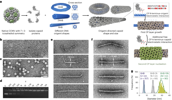
The CPs were isolated from intact CCMV (for virus preparation, see Supplementary Note 21). Briefly, the virus particles were dialysed overnight against 50 mM Tris–HCl, 500 mM CaCl2 buffer, pH 7.5 supplemented with 1 mM dithiothreitol (DTT) using Slize-A-Lyzer Mini Dialysis cups (3.5 kDa MWCO, Thermo Scientific). The RNA was pelleted in a centrifugation step at 4 °C using 21,100g for 6 h, and the recovered supernatant was dialysed overnight against ‘clean buffer’ that contains 50 mM Tris–HCl, 150 mM NaCl at pH 7.5 supplemented with 1 mM DTT (adapted from ref. 60). The concentration of the proteins was determined based on their absorbance at 280 nm (extinction coefficient, 23,590 M-1 cm-1) using a BioTek Eon Microplate Spectrophotometer (2 μl sample, Take3 plate).
ВІК
AGE was used to study the binding interaction between the proteins and the origami structures by monitoring the shift in electrophoretic mobility. Furthermore, the intactness of the origami structures after folding and purification, and during DNase I digestion, was analysed by gel electrophoresis. To this end, samples (volumes ranging from 10 to 32 μl) supplemented with 6× gel loading dye (40% sucrose without dye for samples from digestion studies) were run in a 2% (w/v) agarose gel (1 × Tris–acetate–ethylenediaminetetraacetic acid (TAE) buffer, 11 mM MgCl2) for 45 min at 90 V in 1 × TAE buffer supplemented with 11 mM MgCl2. For staining, ethidium bromide (EtBr) at a final concentration of 0.46 μg ml-1 was used and the DNA was visualized under ultraviolet light using a GelDoc XR+ system (Bio-Rad).
Complexation of DNA origami and CCMV CPs
The complexation between CPs and DNA origami was performed at a final origami concentration of 4 nM (10 μl samples). The origami was added in a 1:1 volume ratio to the protein solution that had been diluted in the ‘clean buffer’. Depending on the required protein excess, ε, which describes the molar ratio between CP to DNA origami, protein solutions ranging from 0 to 60 μM (corresponding to ε = 0–15k) were prepared. The NaCl concentration was adjusted to 150 mM, resulting in a complexation buffer containing 3.25 mM HEPES-NaOH, 25 mM Tris–HCl, 150 mM NaCl and 0.5 mM DTT. The complexation was performed at 4 °C for at least 1 h and subsequently analysed using AGE and TEM.
DNase I digestion assays
To study the protection effect of the CP coating against degradation of the origami structures by DNase I, 2 μl of DNase I stock (ranging from 0 to 500 KU ml-1) was added to 16 μl of the sample. Additionally, CaCl2 and MgCl2 concentrations were adjusted, resulting in a final reaction volume of 20 μl containing 3.2 nM DNA origami, 2.6 mM HEPES-NaOH, 20 mM Tris–HCl, 120 mM NaCl, 0.4 mM DTT, 1 mM CaCl2 and 5 mM MgCl2. The samples are incubated at 37 °C for 15 min (6HB) and 60 min (24HB). Before analysing the outcome by AGE, samples complexed with CPs were disassembled using heparin sodium salt as a competitive binding agent (final concentrations of 1.5 μM for 6HB-2k and 24HB-2.5k and 82 μM for 6HB-10k and 24HB-10k; Supplementary Note 14).
RNA–DNA origami folding and purification
For the RNA–DNA hybrid origami (RNA-6HB), EGFP mRNA (CleanCap EGFP mRNA, TriLink Bio Technologies, L-7601) was used as the scaffold. In a one-pot reaction, the 996-nt-long mRNA scaffold was thermally annealed with 29 staple strands (purchased from Integrated DNA Technologies, see Supplementary Note 22) into a short 6HB structure using a Proflex 3 × 32-well PCR system (Thermo Fisher). The structure is designed to contain two scaffold crossovers and has a helical pitch of 11 bp per turn. For the folding reaction, the mRNA and the staples were diluted into 1 × FOB containing 1 × TAE pH 8.4, 5 mM MgCl2 and 1 mM NaCl reaching final concentrations of 50 nM and 500 nM, respectively. The reaction mixture was incubated at 55 °C for 15 min61 and cooled down by placing it on ice for at least 10 min before storage at 4 °C. To validate the folding, four staple strands were exchanged with staple strands containing a 3′ overhang (labelled with F, Supplementary Table 2). A fluorophore-containing attachment strand (ATTO590, Integrated DNA Technologies), which was added to the folding mixture in 10× excess per attachment site, can then be integrated into the structure by hybridization with the staple overhangs.
The folded structures were purified from excess staple strands by spin-filtration. To this end, the filter (100 kDa MWCO, Amicon) was washed with 400 μl of 1 × FOB by centrifugation at 14,000g for 5 min, followed by two-times addition of 40 μl RNA-6HB together with 40 μl of 1 × FOB. After a centrifugation step at 6,000g for 10 min, 80 μl of 1 × FOB was added and the centrifugation continued (6,000g, 10 min). This washing step was repeated in total three times before the sample was recovered by inverting the filter into a clean tube (1,000g, 2.5 min). The concentration was determined by measuring the absorbance at 260 nm (extinction coefficient, 1.29 × 10⁷ M-1 cm-1), and the successful folding was determined by AGE (3.5 % (w/v) gels, visualization under ultraviolet light (EtBr channel) and red light (A647 channel), ChemiDoc MP system, Bio-Rad), AFM and TEM.
Complexation of RNA-6HB origami and CCMV CPs
For the complexation, purified RNA-6HB origami in 1 × FOB was mixed with CCMV capsids in ‘clean buffer’ in a 1:1 ratio at a final hybrid origami concentration of 7.5 nM. This results in a complexation buffer containing 45 mM Tris, 75.5 mM NaCl, 10 mM acetic acid, 2.5 mM MgCl2, 0.5 mM DTT and 0.5 mM EDTA. The samples were incubated at 4 °C for at least 1 h before analysis with AGE and TEM.
Complexation of DNA origami and NoV CPs
NoVLPs were prepared as reported by Lampinen et al.62 and stored in 1 × phosphate-buffered saline (PBS, 137 mM NaCl, 2.7 mM KCl, 10 mM Na2HPO4 and 1.8 mM KH2PO4, pH 7.4); however, here SpyTag003 (ref. 63) has been fused to the C-terminus of the VP1 from the NoV strain Hu/GII.4/Sydney/NSW0514/2012/AU. The particles were quality controlled with dynamic light scattering for particle formation, sodium dodecyl sulfate polyacrylamide gel electrophoresis for protein purity and the residual dsDNA was measured. For the complexation with DNA origami, DNA origami was present in the sample during both disassembly and reassembly of the VLPs. To this end, the origami structures were transferred into deionized water using spin-filtration (as described above). The DNA origami was mixed with the NoVLPs at different concentrations in a 1:4 (v/v) ratio, resulting in a final origami concentration of 6 nM (30 μl samples). The samples were transferred into 3.5 kDa MWCO dialysis cups (Slize-A-Lyzer, Thermo Scientific) and dialysed overnight at 4 °C against 50 mM Tris–HCl, pH 8.9. For reassembly, the samples were, in a second step, dialysed overnight at 4 °C against 100 mM sodium phosphate buffer, pH 6.0, similarly as reported by White et al.64 The complexation during disassembly and assembly of the NoVLPs was analysed by AGE and TEM.
Complexation of DNA origami and SV40 CPs
The SV40 major CP VP1 (abcam, ab74565) was disassembled and reassembled (adapted from ref. 50) by dialysing the assembled VLPs in PBS against 20 mM Tris, 2 mM DTT, 5 mM EDTA and 50 mM NaCl, pH 8.9 for 2 h at 4 °C (3.5 kDa MWCO, Slize-A-Lyzer, Thermo Scientific), after which the EDTA concentration was decreased by an additional dialysis step at 4 °C for 2 h against 20 mM Tris, 2 mM DTT, 2 mM EDTA and 50 mM NaCl, pH 8.9. The concentration was determined based on the absorbance at 280 nm (VP1 extinction coefficient, 32,890 M-1 cm-1). The DNA origami was transferred into 100 mM HEPES buffer, pH 7.2, supplemented with 125 mM NaCl by spin-filtration (as described above). The proteins were mixed with the DNA origami in 1:1 (v/v) ratio to reach final concentrations of 0–20 μM and 2 nM, respectively, and the samples were incubated for 24 h at room temperature before analysis using AGE and TEM.
Complexation of DNA origami and MPyV CPs
For the complexation of VP1 capsomers (for recombinant expression and purification, see Supplementary Note 23) and DNA origami, the origami structures were first transferred into 40 mM Tris buffer, pH 8.0, supplemented with 20 mM acetic acid, 2 mM EDTA and 12 mM MgCl2 using spin-filtration (see above). Depending on the desired excess of proteins, ε, the capsomers were diluted into ‘storage buffer’, containing 40 mM Tris, 200 mM NaCl, 1 mM EDTA, 5% (v/v) glycerol and 5 mM DTT, pH 8.0. For the complexation, VP1 capsomers were diluted in a ratio of 1:20 in the origami solution, resulting in a final origami concentration of 0.75 nM (30 μl samples) and a complexation buffer containing 40 mM Tris, 19 mM acetic acid, 1.95 mM EDTA, 11.4 mM MgCl2, 10 mM NaCl, 0.25% (v/v) glycerol and 0.25 mM DTT, pH 8. The complexation reaction was incubated at 4 °C overnight before analysis with AGE and TEM.
AFM
A 20 μl droplet of 10 nM RNA-6HB origami solution (MgCl2 concentration adjusted to 12.5 mM) was deposited on a freshly cleaved mica substrate (Electron Microscopy Sciences) for 1 min, followed by three washing steps with 100 μl deionized water that was immediately blotted away. The sample was dried under a steady nitrogen stream and imaged immediately after sample preparation. AFM images were acquired in air using ScanAsyst in Air Mode together with ScanAsyst-Air probes (Bruker) on a Dimension Icon AFM (Bruker). Image processing was performed in NanoScope Analysis v.1.90 (Bruker).
TEM
Plain DNA origami samples (4 nM) were prepared by incubation of a 3 μl droplet for 3 min on a plasma cleaned (20 s oxygen plasma flash, Gatan Solarus) Formvar carbon-coated copper grid (FCF400Cu, Electron Microscopy Sciences), which was subsequently blotted against filter paper and negative stained. For CCMV-CP-complexed samples (4 nM DNA origami), a 3 μl droplet was deposited on the grid for 1.5 min. After blotting against filter paper, the grid was immersed in a 10 μl droplet of complexation buffer (3.25 mM HEPES-NaOH, 25 mM Tris–HCl, 150 mM NaCl, 0.5 mM DTT) for 5 s. For samples with DNA origami concentrations ≤2 nM (for example, complexation with SV40, MPyV), and for samples containing RNA-6HB (7.5 nM origami concentration), the droplet size was increased to 5 μl and the incubation time extended to 5 min. Negative staining65 was performed by first immersing the grid in a 5 μl droplet of aqueous 2% (w/v) uranyl formate solution (supplemented with 25 mM NaOH for pH adjustment), which was immediately blotted away. This step was followed by an immersion in a 20 μl droplet, which was incubated on the grid for 45 s. After the final blotting step, the samples were left to dry for at least 20 min before imaging was performed on a FEI Tecnai 12 Bio-Twin microscope at an acceleration voltage of 120 V.
Кріо-ЕМ
The samples for cryo-EM were prepared using a vitrification apparatus (Vitrobot, Thermo Fisher Scientific). The origami concentrations in the complexed samples were 90 nM for 6HB-2k, 84 nM for 24HB-2.5k, 18 nM for 6HB-10k and 21 nM for 24HB-10k, resulting in total CP concentrations of 180 μM and 210 μM for complexed 6HB and 24HB samples, respectively. A 3 μl aliquot of the complexed origami sample was deposited on a plasma-cleaned (50 s, Harrick Plasma PDC-002-EC instrument) holey carbon-coated grid (copper 200 mesh R1.2/1.3, Quantifoil). After a 1 min incubation, excess liquid was blotted for 10 s at 100% relative humidity and 6 °C, followed by plunging the grid into liquid ethane. The grids were stored in liquid nitrogen. Data were collected at liquid nitrogen temperature in a Talos Arctica transmission electron microscope (Thermo Fisher Scientific) operated at 200 kV, using a Falcon III direct electron detector (Thermo Fisher Scientific). A magnification of 150,000× was used, resulting in a calibrated pixel size of 0.96 Å. The data collection parameters are listed in Supplementary Table 4 (Додаткова примітка 24).
Single-particle reconstruction
Cryo-EM data were processed using CryoSPARC 3.3.2 (Structura Biotechnology) unless stated otherwise. Contrast transfer function parameters were estimated using CTFFIND4 (ref. 66). Segments along filaments were defined using the Filament Tracer function. Helical symmetry parameters were estimated initially from 2D class averages using Python-based Helix Indexer67. The structure and helical symmetry parameters were refined using Helix Refine function and non-uniform refinement on motion-corrected helix segments. To determine the helical symmetry parameters of the 6HB-10k outer layer, a second 2D classification run was performed after subtracting the contribution of the inner layer using the Particle Subtraction function. The Helix Refine was run on the subset of particles that showed a clear second layer, using the determined symmetry parameters as initial estimates. Reconstructions were sharpened by applying an ad hoc B-factor of −300 Å2. The reconstructions were averaged in real space by imposing the helical symmetry parameters on the central, most ordered part of the map (50% of the volume) in Bsoft68.
For modelling the structure of the capsomer, CP monomer (PDB:1cwp) was fitted in the 6HB-2k reconstruction in the six positions of the hexamer as rigid bodies in UCSF ChimeraX 1.3 (ref. 69). The atomic model was refined against the density using ISOLDE 1.3 (ref. 70) and Phenix 1.19 (ref. 71). To create atomic representations of the filaments, symmetry copies of the hexamer were created in ChimeraX. To visualize the placement of CP hexamers and pentamers in the cap, the caps of the 6HB-2k filament were manually picked in the micrographs. The cap structure was refined using the Helix Refine function omitting symmetrization, as this allowed limiting the tilt angle of the caps close to side views. Reconstruction of the cap was filtered to its local resolution using Local Filter. The hexamer atomic model and previously determined pentamer structure (extracted from PDB:1cwp after applying icosahedral symmetry) were fitted as rigid bodies in ChimeraX 1.3. Data-processing parameters are given in Supplementary Table 4. Model refinement and validation parameters are shown in Supplementary Table 5.
SAXS
The samples for SAXS were prepared at origami concentrations of 165 nM (6HB, corresponding to a disassembled CP concentration of 330 μM) and 180 nM (24HB, corresponding to a disassembled CP concentration of 450 μM) and sealed within a 1.5-mm-diameter glass capillary. The measurements were performed using a Xenocs Xeuss 3.0C device equipped with a GeniX 3D copper microfocus source (wavelength λ = 1.542 Å) and an EIGER2 R 1M hybrid pixel detector at a sample–detector distance of 1,100 mm. Data acquisition was performed for 3 × 3 h per sample. To obtain the 1D SAXS data, the 2D scattering data were azimuthally averaged. The magnitude of the scattering vector q дається (q,=,4uppi sin theta /lambda) з 2θ being the scattering angle. Data treatment included averaging of the triplicate 2D data of each sample, background subtraction from the complexation buffer (3.25 mM HEPES-NaOH, 25 mM Tris–HCl, 150 mM NaCl, 0.5 mM DTT) and a form factor was fitted to a cylinder (6HB, 24HB), spheres (T = 3 icosahedral CPs assemblies) and a core–shell cylinder (6HB-2k, 24HB-2.5k) using SasView software. A Debye–Anderson–Brumberger model was added to account for the background.
- Розповсюдження контенту та PR на основі SEO. Отримайте посилення сьогодні.
- PlatoData.Network Vertical Generative Ai. Додайте собі сили. Доступ тут.
- PlatoAiStream. Web3 Intelligence. Розширення знань. Доступ тут.
- ПлатонЕСГ. Автомобільні / електромобілі, вуглець, CleanTech, Енергія, Навколишнє середовище, Сонячна, Поводження з відходами. Доступ тут.
- BlockOffsets. Модернізація екологічної компенсаційної власності. Доступ тут.
- джерело: https://www.nature.com/articles/s41565-023-01443-x
- : має
- :є
- ][стор
- 1
- 1: співвідношення 1
- 1.3
- 10
- 100
- 11
- 116
- 12
- 14
- 15%
- 16
- 180
- 19
- 1M
- 2%
- 20
- 200
- 2011
- 2014
- 2015
- 2018
- 2019
- 2021
- 2022
- 2023
- 23
- 24
- 25
- 27
- 2D
- 30
- 31
- 32
- 3d
- 40
- 46
- 50
- 500
- 60
- 65
- 66
- 67
- 7
- 70
- 75
- 8
- 80
- 84
- 9
- 90
- a
- вище
- прискорення
- рахунки
- точний
- придбаний
- придбання
- Ad
- пристосований
- доданий
- доповнення
- Додатковий
- Додатково
- Відрегульований
- Регулювання
- після
- проти
- вік
- Агент
- AIR
- AL
- дозволено
- по
- an
- аналіз
- Якір
- та
- Застосування
- наближається
- ЕСТЬ
- навколо
- AS
- зібраний
- збірка
- At
- усереднення
- геть
- фон
- заснований
- BE
- було
- перед тим
- буття
- між
- обов'язковий
- біотехнології
- органів
- обидва
- BP
- коротко
- буфера
- Створюємо
- by
- CAN
- кришка
- шапки
- Клітини
- стільниковий
- центральний
- Канал
- вибір
- клас
- класифікація
- ясно
- клацання
- близько
- збір
- конкурентоспроможний
- концентрація
- Умови
- містить
- триває
- контрастність
- внесок
- контроль
- copies
- Мідь
- Відповідний
- створювати
- створений
- дані
- обробка даних
- певний
- доставка
- Щільність
- Залежно
- депонований
- описаний
- призначений
- бажаний
- Визначати
- певний
- розробників
- пристрій
- Діаліз
- різний
- Розмір
- прямий
- відстань
- ДНК
- вниз
- висушити
- під час
- динамічний
- e
- E&T
- кожен
- ed
- педагогів
- ефект
- кінець
- Машинобудування
- забезпечувати
- Навколишнє середовище
- рівним
- обладнаний
- оцінка
- Оцінки
- Ефір (ETH)
- приклад
- надлишок
- обмін
- обмінялися
- вираз
- вимирання
- фактор
- сокіл
- ШВИДКО
- fei
- фільтрувати
- Фільтри
- остаточний
- виявлення
- Перший
- спалах
- потім
- для
- форма
- освіта
- чотири
- від
- функція
- Крім того
- даний
- скло
- поступово
- сітка
- Зростання
- керівні вказівки
- було
- тут
- Високий
- Однак
- HTTPS
- гібрид
- i
- ICE
- ICON
- III
- зображення
- зображень
- Зображеннями
- негайно
- занурений
- занурення
- накладення
- in
- включені
- збільшений
- інкубований
- ІНКУБАЦІЯ
- індексатор
- початковий
- спочатку
- інструмент
- інтегрований
- взаємодія
- інтерфейс
- в
- Іонний
- ізольований
- IT
- ЙОГО
- КДА
- шар
- найменш
- залишити
- світло
- LINK
- Рідина
- Перераховані
- погрузка
- місцевий
- основний
- вручну
- карта
- карти
- матеріал
- виміряний
- вимірювання
- вимір
- сітці
- методика
- Слюда
- Мікроскоп
- Мікроскопія
- хвилин
- змішаний
- суміш
- мобільність
- режим
- модель
- моделювання
- модульний
- MOL
- молекулярний
- моніторинг
- найбільш
- мРНК
- нано
- нанотехнології
- природа
- негативний
- отримувати
- of
- on
- працювати
- оптимізований
- інакше
- Результат
- за ніч
- Кисень
- Папір
- параметри
- частина
- частинка
- PBS
- PCR
- для
- виконується
- Фізично
- підібраний
- Крок
- піксель
- розміщення
- Плазма
- платформа
- plato
- Інформація про дані Платона
- PlatoData
- занурюючись
- позиції
- підготовка
- підготовлений
- представити
- раніше
- Праймер для вій
- ПРОЦ
- Процедури
- оброблена
- обробка
- програма
- захист
- Білок
- Білки
- придбано
- якість
- ранжування
- співвідношення
- досягати
- досягнення
- реакція
- реальний
- реалістичний
- червоний
- удосконалювати
- рафінований
- про
- відносний
- повторний
- Повідомляється
- вимагається
- Дослідники
- дозвіл
- відповідно
- в результаті
- результати
- жорсткий
- РНК
- Кімната
- прогін
- s
- сіль
- SCI
- НАУКИ
- науковий
- другий
- побачити
- сегменти
- зсув
- Короткий
- показав
- показаний
- сторона
- Аналогічно
- сайт
- SIX
- Розмір
- менше
- натрій
- Софтвер
- рішення
- Рішення
- Source
- Простір
- розкол
- заявив,
- стійкий
- Крок
- заходи
- акції
- зберігання
- зберігати
- Пасма
- потік
- сила
- структура
- Дослідження
- Вивчення
- Згодом
- успішний
- система
- таблиця
- талори
- Технології
- Що
- Команда
- їх
- потім
- Theta
- це
- три
- через
- час
- times
- до
- разом
- інструмент
- Усього:
- ізотопний індикатор
- переклад
- передані
- лікування
- ПЕРЕГЛЯД
- два
- при
- USA
- використання
- використовуваний
- користувач
- Інтерфейс користувача
- використання
- Вакцина
- ПЕРЕВІР
- перевірка достовірності
- різнобічний
- думки
- вірус
- візуалізації
- Напруга
- обсяг
- Обсяги
- W
- було
- мийка
- вода
- вага
- були
- який
- білий
- з
- в
- без
- X
- врожайність
- зефірнет