Single-molecule analysis of DNA base-stacking energetics using patterned DNA nanostructures – Nature Nanotechnology

Slide preparation

Microscopy slide and coverslip preparation was done as previously described^39,43. The slides (VWR 631-1550) were drilled using a diamond head drill bit (Meisinger 801-009-HP) and drill gun (DigitalCraft LRUXOR). In case the slides were being reused, macroscopic particles were removed using 5% v/v dish washing detergent before further steps were performed. Slides and coverslips (VWR 631-0147) were initially rinsed thoroughly using MilliQ water and then immersed into coplin jars (Tarsons 480000) containing MilliQ water. The slides and coverslips were then sonicated for 5 min (IGene LabServe IGNUC-9). MilliQ water was then replaced with acetone (SRL 31566) twice and was sonicated for 5 min. Acetone was then replaced with MilliQ water followed by 1 M KOH (BDH 296228) and sonicated for at least 30 min. The slides and coverslips were then rinsed using MilliQ water by replacing the KOH in the coplin jars at least three times. The slides and coverslips were then sonicated in MilliQ water for 10 min and dried using compressed nitrogen gas.

Piranha etching was performed on the slides and coverslips. Piranha solution was prepared by adding one part of 30% H₂O₂ (EMPLURA 107209) to three parts of H₂SO₄ (Fisher Scientific 29997). This solution was then transferred into the coplin jars and left for 30 min. The piranha solution was disposed of in a dedicated waste container, and the slides and coverslips were rinsed thoroughly using MilliQ water, then rinsed with methanol twice and sonicated in methanol for 20 min.

After this, aminosilanation was performed. The aminosilanation mix was prepared by mixing 5 ml acetic acid (SDFCL 20001) in 100 ml methanol, followed by addition of 10 ml (3-aminopropyl) triethoxysilane (SRL 33993 or TCI A0439) and mixed thoroughly. This solution was then poured over the slides and coverslips held within the coplin jar and left for 25 min. The slides and coverslips were washed thoroughly with fresh methanol three times followed by rinsing with MilliQ water. Slides were then dried with compressed nitrogen gas.

Passivation was performed on these aminosilanated slides using mPEG-SVA (succinimidyl valerate) (Laysan Bio mPEG-SVA-5000) and biotin-PEG-SVA (Laysan Bio Biotin-PEG-SVA-5000) at a 40:1 mass ratio in 0.1 M NaHCO₃ (Sigma S5761) pH 8.5. For 15 pairs of slides and coverslips, 120 mg mPEG-SVA and 3 mg biotin-PEG-SVA were dissolved in 960 µl of 0.1 M NaHCO₃. Then 60 µl of this solution was added onto each slide and then sandwiched by placing a coverslip over it gently. These slides and coverslips were stored in humid chambers for 8–12 h at room temperature (21 °C) under dark. The following day, the sandwich was disassembled and washed thoroughly with MilliQ water. These slides were then dried with compressed nitrogen gas and stored inside 50 ml centrifuge tubes (NUNC 339653) and stored under inert conditions in nitrogen gas.

The flow cells were assembled using double-sided tape (3 M Scotch 136D MDEU) on the PEG-passivated surface of the sides. Coverslips were placed on the taped slide ensuring that the PEG-passivated surfaces of the slide and coverslip make up the interiors of the microfluidic flow cells. The open edges of these channels were sealed using epoxy (Araldite Klear).

DNA-origami folding

We used the Picasso design module³³ to get the staple sequences of specific extensions for the grids and blank staples (Supplementary Table 8, sheets 1 and 2) for preparing rectangular DNA-origami nanostructures. M13mp18 single-stranded DNA (Bayou Biolabs P107) was used as the scaffold for the DNA origami. Biotinylated oligonucleotide staples (Supplementary Table 8, sheet 3) were used to anchor the origami structure to the flow cell surface. Staples with extension for the gap and nick positions were designed using sequences from Picasso design and CadNanoSQ (https://cadnano.org/; Supplementary Table 8, sheets 4 and 5). Folding buffer contained 50 mM Tris-Cl (Tris-Base, Sigma 77861; HCl, Fisher Scientific 29507) pH 8.0, 12.5 mM MgCl₂ (EMPLURA 105833) and 0.2 mM EDTA (SRL 35888). We set up 30 µl reactions with 10 nM scaffold DNA, 100 nM biotin staples, 100 nM blank staples, 1 µM staples for the grid and 33.3 µM gap- or nick-specific staple in the folding buffer. The mix was then heated up to 80 °C, held for 5 min, and then cooled to 4 °C, in steps of 0.1 °C every 5 s in a thermocycler.

The folded origami structures were purified using Sartorius Vivaspin 500 (Sartorius VS0132) centrifugal filters. Equilibration was performed by spinning the columns at 3,000g for 5 min with 500 µl HPLC-grade water (SRL 92605) followed by 500 µl folding buffer. The resultant origami mix was then applied to the column along with 500 µl folding buffer at 800–1,000g for three rounds, to remove most of the unincorporated staples. Origami structures were stored in the folding buffer at a concentration of 3.3 nM at −20 °C.

Imager fluorophore conjugation and purification

We obtained 3′-end amine modified oligonucleotides from Sigma (Supplementary Table 8, sheet 6) and dissolved to a final concentration of 1 mM using HPLC-grade water.

Fluorophores were dissolved in DMSO (Sigma D8418) to the following concentrations. Cy3B-MonoNHS-Ester (Cytiva PA63101) was dissolved to a final concentration of 13 mM, Atto647N-MonoNHS-Ester (Sigma 18373-1MG-F) was dissolved to a final concentration of 11.8 mM and Cy5-MonoNHS-Ester (Cytiva PA15101) was dissolved to a final concentration of 1.3 mM.

A 10× PBS was prepared by adding 80 g NaCl (SRL 3205), 2 g KCl (Sigma P9541-1KG), 14.4 g Na₂HPO₄ (SRL 1949146) and 2.4 g KH₂PO₄ (Ranbaxy 5HEV0740) in 1 l of MilliQ water followed by autoclaving at 121 °C for 15 min. The pH of the buffer was adjusted to 7.4.

For conjugation of Cy3B or Atto647N to the imager, 15 nM DNA (15 µl from 1 mM stock) was dissolved in a mixture containing 3 µl 10× PBS, 3 µl of 1 M NaHCO₃ and 3.24 µl HPLC-grade water. Seventy-five nanomoles (5.76 µl of 13 mM Cy3B or 6.35 µl of 11.8 mM Atto647N) of fluorophore was added to the above mixture and vortexed vigorously. The mix was incubated overnight in the dark at room temperature under vigorous shaking.

For conjugation of Cy5 to the imager, 2 nM DNA (2 µl from 1 mM stock) was dissolved in a mixture containing 1.5 µl 10× PBS, 1.5 µl of 1 M NaHCO₃ and 4 µl HPLC-grade water. Then 7.8 nM (6 µl of 1.3 mM Cy5) fluorophore was added to the above mixture and vortexed vigorously. The mix was incubated overnight in the dark at room temperature under vigorous shaking.

Post overnight incubation, the conjugated product was purified from the free fluorophore and unconjugated DNA oligonucleotide using reverse-phase (Phenomenex 00B-4442-E0 Clarity 5 µm Oligo-RP, LC column 50 × 4.6 mm, Ea) HPLC (Agilent Technologies). The conjugated product was then dissolved in HPLC-grade water and stored at −20 °C.

Sample preparation

Microfluidic flow cells with a PEG-passivated coverslip and slide were incubated with 10 µl of 0.2 mg ml⁻¹ neutravidin (Sigma 31000) in T50 buffer containing 50 mM Tris-Cl pH 8.0, 50 mM NaCl and 0.2 mM EDTA for 20 min. This was followed by thorough washing of the microfluidic channel with 600 µl of T50 buffer. Imaging/immobilization buffer (buffer I) containing 50 mM Tri-Cl pH 8.0, 10 mM MgCl₂ and 0.2 mM EDTA was used to wash the channel before origami immobilization. The origamis intended for a specific imaging run were pooled together at a final concentration of 400–600 pM each in buffer I and applied onto the channel and incubated for 20 min. This was followed by washing of the channel with 600 µl buffer I before imaging to remove any unbound origamis.

Microscopy and imaging

Microscopy was performed on a Nikon Ti2 Eclipse microscope equipped with a motorized H-TIRF, perfect focus system and a Teledyne Photometrics PRIME BSI sCMOS camera. Illumination using 561 nm and 640 nm wavelength lasers was done using the L6cc laser combiner from Oxxius. Imaging was done under total internal reflection conditions. An oil immersion objective lens (Nikon Instruments Apo SR TIRF 100×, numerical aperture 1.49, oil) was used for imaging. Imaging was performed with 2 × 2 binning of pixels and the camera was cropped to an effective size of 512 × 512 pixels, each pixel spanning 130 × 130 nm. Acquisition was done by setting the camera to a readout sensitivity of 16 bit. Imaging parameters used in the different experiments are outlined in Supplementary Table 7.

A solution of 20× PCD was made by dissolving PCD (protocatechuate 3,4-dioxygenase; Sigma P8279-25UN) in buffer containing stock in 50 mM KCl, 1 mM EDTA and 100 mM Tris–HCl, pH 8.0 and 50% glycerol (Sigma G5516-1L) to a final concentration of 6 µM. The solution was divided into 10 µl aliquots in PCR tubes and stored at −20 °C.

A solution of 40× PCA was made by dissolving 154 mg of PCA (protocatechuic acid/3,4-dihydroxybenzoic acid; Sigma 37580-100G-F) in 10 ml HPLC-grade water adjusted to pH 9.0 using 1 M NaOH (SRL 96311). The solution was divided into 100 µl aliquots in 200 µl tubes and stored at −20 °C.

A solution of 100× trolox was prepared by dissolving 100 mg of trolox (6-hydroxy-2,5,7,8-tetramethylchroman-2-carboxylic acid; Sigma 238813-1 G) in 430 µl methanol, 345 µl of 1 M NaOH and 3.2 ml HPLC-grade water. The solution was divided into 20 µl aliquots in PCR tubes and stored at −20 °C.

Before imaging, 100 µl of imaging buffer was prepared in buffer I with a final concentration of 1× PCA, 1× PCD and 1× trolox, along with imagers at concentrations mentioned in Supplementary Table 7. Imaging was always performed with the 640 nm laser before the 561 nm laser to minimize the effect of Atto647N or Cy5 fluorophore photobleaching by the higher-energy (561 nm) light source.

Imaging of stem-loop layout

Origamis were folded in the same manner as mentioned above (Supplementary Table 8, sheets 1 and 7–9). Imaging was performed using Exchange-PAINT⁵⁴, where the first round of imaging was done to image the origamis carrying R1×5 extensions followed by origamis carrying R4×5 extensions with appropriate imagers carrying Atto647N fluorophore at the mentioned concentrations (Supplementary Table 7). Imaging buffer was prepared as mentioned above. Subsequent imaging rounds were separated by washing with 2 ml imaging buffer. Finally, the nick and gap were measured using Cy3B-labelled imager at the concentrations mentioned in the Supplementary Table 7.

Data analysis

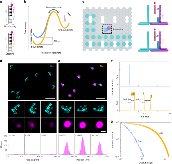
The obtained raw fluorescence data were reconstructed using the Picasso Localize software package³³ to obtain a super-resolved image. Drift correction in X–Y was performed by redundant cross-correlation. Redundant cross-correlation was also used to align the super-resolved structures from the two imaging channels (Supplementary Fig. 1). Origamis were manually picked based on their grid structures. Localizations from the gap or nick spots from the assay sites were extracted using Picasso Render for further kinetics analysis. We performed kinetic analysis using a custom-written MATLAB code. Briefly, the list of localizations exported for each origami pick was further analysed for individual dwell times and dark times. Dwell times were calculated based on the presence of consecutive binding events with a gap of not more than 25 frames (that is, 1,250 ms; Fig. 1f). This is done to overcome any potential flickering of the fluorophore and the lower signal-to-noise ratios that arise due to the lower laser powers that were used during imaging to maintain the photostability of the fluorophore (Supplementary Fig. 8). Further, this will unlikely combine two consecutive binding events due to the long time intervals of around 100 s to 200 s between consecutive bindings (Supplementary Fig. 9). Bootstrapping for 100 iterations was performed based on the mean using MATLAB’s built-in bootstrap function on the list of individual dwell times for each dataset separately.

Dark times were calculated based on the durations between two consecutive binding events (Fig. 1f). The obtained dark times were bootstrapped with parameters mentioned above and used for further kinetic analysis.

Kinetic analysis for calculating the base-stacking energies

Here we describe the kinetic analysis of the single-molecule imaging data. The set of bootstrapped dwell times were plotted on histogram and then fit with a mono-exponential curve ((y={a}_{1}times {{mathrm{e}}}^{{k}_{{{mathrm{off}}}}{t}})) in case of the gap, resulting in the off-rate constant k_off,gap. For the nick configuration data, we fit them with a bi-exponential curve ((y={a}_{1}times {{mathrm{e}}}^{{k}_{{{{mathrm{off}}}}{,1}}{t}}+{a}_{2}times {{mathrm{e}}}^{{k}_{{{{mathrm{off}}}}{,2}}{t}})) using gap off-rate as proxy for fitting the first exponential. The distribution of individual dwell times shown in Supplementary Fig. 4a clearly shows that the imager binds on the docking strand in two modes—one without the terminal nucleotide stacking on the stem, leading to a faster decaying population, and the second with terminal nucleotides stacking, leading to a slower decaying population away from the first population (Supplementary Fig. 4a). As we observed two distinct populations in the individual dwell-time distributions, we assumed that the unstacked binding mode was due to the stem undergoing fraying temporarily; the mechanistic details behind this are still unclear, although similar observations have been reported by other studies^41,42. The fraying of the stem is mechanistically equivalent of the gap construct. This fitting results in two off-rate constants (k_off,1 and k_off,2) in which k_off,1 denotes the dissociation from unstacked-bound state to the unbound state, which closely resembles the gap off-rate constant. The second off-rate constant, k_off,2, depicts the imager’s apparent dissociation rate from the bound state, which comprises of bound-stacked and bound-unstacked states to the unbound state (Supplementary Fig. 5). This kinetic analysis provides us with the off-rate constants of unstacked- and stacked-bound states based on the experimentally measured dwell times.

In a similar manner, we also obtained the binding rate constant (k_bind) by kinetic analysis of the dark-time distributions. We built a histogram of the bootstrapped dark times and fit with a mono-exponential curve ((y={b}_{1}times {{mathrm{e}}}^{{k}_{{{mathrm{bind}}}}{t}})) to obtain the individual binding rate constants for the gap and the nick configurations.

The gap configuration is modelled with a bound state and an unbound state with corresponding binding rate (k_bind,gap) and dissociation rate (k_off). On the nick configuration, imager binding is represented by rate constant k_bind in the ‘frayed’ stem state or the intact state. The frayed state resembles the gap configuration. When the stem is intact, the imager binds in either the stacked or the unstacked state with rate constants k_on,st and k_on,unst, respectively. Once in the bound state, the imager may undergo stacked-to-unstacked transitions and vice versa as indicated within the binding event; while doing so, the imager may dissociate from either the stacked or the unstacked configuration with rate constants represented by k_off,st and k_off,unst, respectively (Supplementary Fig. 5). We have neglected the stacked-unpaired and the unstacked-unpaired states (both of which trigger dissociation) whose occupancies would be relatively low.

The apparent rate of dissociation (k_off,2) from the bound state can be written as

where N_st and N_unst are occupancies of stacked and unstacked states during the bound state.

k_off,st is rate of dissociation from the stacked state and k_off,unst is the rate of dissociation from the unstacked state.

Assuming that k_off,st is very slow compared with k_off,2, we discard k_off,st in the denominator. That provides us with the following equation.

We are assuming that k_off,unst and k_off,gap are equivalent, which is a reasonable assumption because the imager in both configurations carry the same base pairs without terminal nucleotides stacking and we experimentally obtained k_off,gap. We also have obtained k_off,2 from experiments, which is the dissociation rate from the bound state.

Hence

This ratio of stacked-to-unstacked occupancies in the bound configuration can be converted to the free energy of base stacking by taking Boltzmann’s weightage over it.

Therefore, the free energy of dinucleotide base stacking is given by the following equation.

where k is the Boltzmann constant and T is the absolute temperature.

Plugging equation (1) in to equation (2) provides us the free energy of base stacking.

We calculated all the dinucleotide stacking free energies using the above equation. We note that a similar formalism was applied by ref. ³ for extracting the stacking free energies after gel electrophoresing of gapped, nicked and intact DNA molecules.

Note that the ΔG_stack is independent of the imager concentration as it only depends on the off-rate constants. The absolute temperature T is constant. If the temperature, concentration and salinity of the buffer in independent experiments are not well controlled, larger variations are expected in the free-energy estimations as the binding dynamics of short oligonucleotides are strongly dependent on these parameters⁴⁰. The multiplexed experiments utilized in the current study are resistant to such possible variations as the normalization is internal to individual imaging experiments.

Photobleaching calculation

Origamis carrying the S1 docking sequence (Supplementary Table 8, sheet 10) were folded using methods mentioned above. DNA origamis were immobilized on flow cells treated with neutravidin as mentioned above. Complimentary S1 strand carrying Cy3B was flown in at 1 pM concentration in buffer I. After 10 min of incubation, the flow cells were washed with 1 ml of buffer I to remove any unbound complimentary S1 strands carrying Cy3B. Imaging buffer was prepared with 1× PCA, 1× PCD and 1× trolox. For recreating the exact same conditions of the Cy3B imaging round (second imaging round), the imaging buffer was added to the flow channel and a dummy imaging run was performed for the duration of the first imaging rounds. This was followed by imaging of the stably bound Cy3B with 561 nm laser excitation in TIRF mode at a similar power to the experiments depicted in Fig. 3 and mentioned in Supplementary Table 7.

The acquired image was run through the Picasso Localize³³ package to track individual fluorophores over a time course. Individual photobleaching times were obtained from the time traces generated similar to image analysis described above. These individual bleaching times were then plotted in a histogram. The fluorophores surviving throughout the imaging run and a small population of fluorophores that bleach during the first 100 s (first bin in Supplementary Fig. 8) were ignored for exponential fitting. The plotted events were then fit with a mono-exponential curve ((y={atimes }{{mathrm{e}}}^{{k}_{{{mathrm{photobleach}}}}{t}})) to obtain the photobleaching rate.

Tetrahedron folding and analysis

The tetrahedron origami structures are composed of three different DNA strands, namely L, M and S^30,51. These strands were designed to carry different stacking ends (Fig. 4a). The sequences of strands L, M and S are shown in Supplementary Table 5. These strands were pooled in the order shown in Supplementary Table 6 in a 1:3:3 ratio. The pooled mixtures were heated to 95 °C and let to cool over a period of 48 h in an insulated water tub in 1× TAE/Mg²⁺ buffer composed of 40 mM Tris, pH 8.0, 20 mM acetic acid, 2 mM EDTA and 12.5 mM magnesium acetate. The structures were then stored at −20 °C. The samples were thawed at room temperature 20 min before loading on the gel. A 1-mm-thick 4% polyacrylamide gel (29:1) prepared in 1× TAE/Mg²⁺ buffer was used for analysing structure formation. Then 20 µl of sample along with 5 µl loading dye containing 0.003% bromophenol blue and 60% glycerol in 1× TAE/Mg²⁺ buffer was loaded in each well. For size reference, a 50 bp plus DNA ladder (dxbidt R4006) that was diluted by 20 times in 1× TAE/Mg²⁺ buffer before loading was used. The gels were run at constant voltage for 120 min at 4 °C in a cold room. The gels were then stained using GelRed (Biotium 41003) stain diluted to 3× in 0.1 M NaCl solution for 30 min on a gel rocker. The gels were then visualized in an ultraviolet transilluminator and quantified using BioRad Image Labs 6.1.

Quantification of the fraction of assembled tetrahedron was performed by dividing the tetrahedron band intensity by the total intensity of the same lane after background subtraction. The obtained values were then normalized with the greatest obtained fraction to quantify the fraction of assembled tetrahedron in each experimental triplicate.

Stack-PAINT imaging

Origami structures were folded with staples defined in Supplementary Table 8, sheet 11, and purified using centrifugal filtration. The origami samples were immobilized on the surface of a PEG-passivated glass slide as described above. Imaging was performed as mentioned in Supplementary Table 7. Reconstructed data were aligned for both channels. Origamis were picked based on the six extensions that were placed for resolution testing and then filtered based on the presence of the underlying grid. The mean dwell times at each picked origami structure was calculated. We then constructed a histogram from the mean dwell times and fitted with a triple Gaussian curve using the MATLAB ‘gauss3’ function. Each of the three Gaussian peaks was split into three datasets by manual demarcation based on the known dwell-time averages over each pick. For assessing the robustness of our decoding technique, we manually filtered the selected origami structures based on the grid structures. We then compared the manual selection set with the set delineated based on the average dwell times. We calculated the error in calling the correct origami by taking the ratio of origami numbers that fall outside the expected region to total origami structures analysed.

Statistics and reproducibility

No statistical method was used to predetermine the sample size. Each stacking experiment was performed in triplicate. As evident from the data, the results were highly reproducible.

• SEO Powered Content & PR Distribution. Get Amplified Today.
• PlatoData.Network Vertical Generative Ai. Empower Yourself. Access Here.
• PlatoAiStream. Web3 Intelligence. Knowledge Amplified. Access Here.
• PlatoESG. Automotive / EVs, Carbon, CleanTech, Energy, Environment, Solar, Waste Management. Access Here.
• PlatoHealth. Biotech and Clinical Trials Intelligence. Access Here.
• ChartPrime. Elevate your Trading Game with ChartPrime. Access Here.
• BlockOffsets. Modernizing Environmental Offset Ownership. Access Here.
• Source: https://www.nature.com/articles/s41565-023-01485-1