Mastering The Art Of Data Cleaning In Python - KDnuggets

Republished By Plato

Followers: 0

Mastering the Art of Data Cleaning in Python

Image by Author

Data cleaning is a critical part of any data analysis process. It's the step where you remove errors, handle missing data, and make sure that your data is in a format that you can work with. Without a well-cleaned dataset, any subsequent analyses can be skewed or incorrect.

This article introduces you to several key techniques for data cleaning in Python, using powerful libraries like pandas, numpy, seaborn, and matplotlib.

Before diving into the mechanics of data cleaning, let's understand its importance. Real-world data is often messy. It can contain duplicate entries, incorrect or inconsistent data types, missing values, irrelevant features, and outliers. All these factors can lead to misleading conclusions when analyzing data. This makes data cleaning an indispensable part of the data science lifecycle.

We’ll cover the following data cleaning tasks.

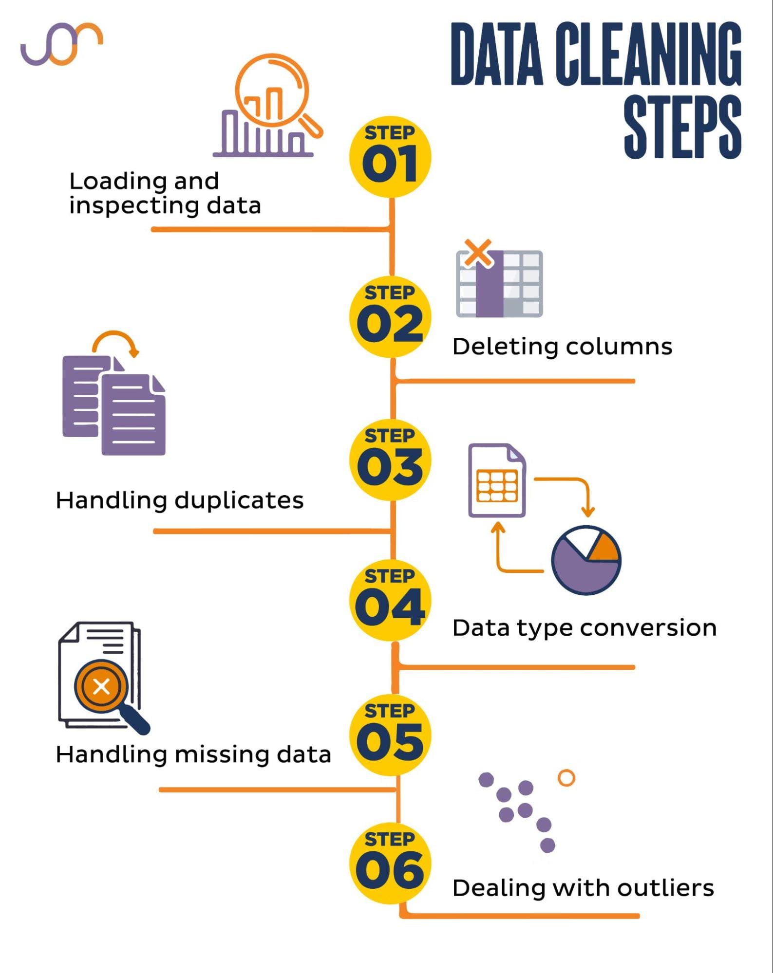
Image by Author

Before getting started, let's import the necessary libraries. We'll be using pandas for data manipulation, and seaborn and matplotlib for visualizations.

We’ll also import the datetime Python module for manipulating the dates.

import pandas as pd
import seaborn as sns
import datetime as dt
import matplotlib.pyplot as plt
import matplotlib.ticker as ticker

First, we'll need to load our data. In this example, we're going to load a CSV file using pandas. We also add the delimiter argument.

df = pd.read_csv('F:KDNuggetsKDN Mastering the Art of Data Cleaning in Pythonproperty.csv', delimiter= ';')

Next, it's important to inspect the data to understand its structure, what kind of variables we're working with, and whether there are any missing values. Since the data we imported is not huge, let’s have a look at the whole dataset.

# Look at all the rows of the dataframe
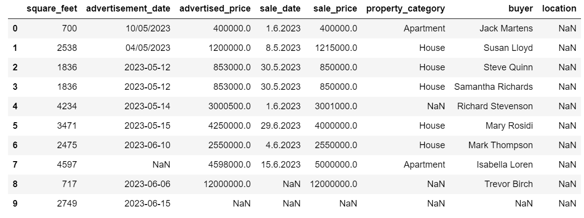
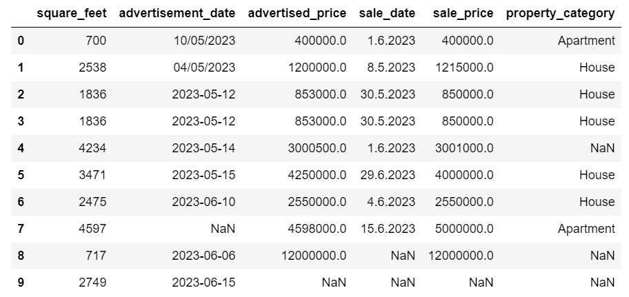
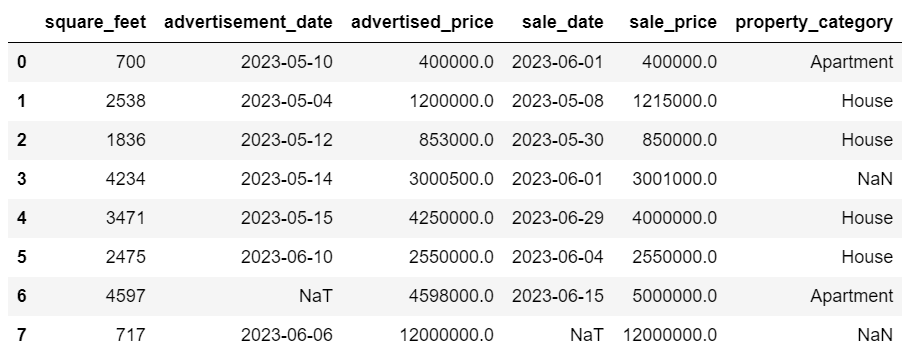
display(df)

Here’s how the dataset looks.

You can immediately see there are some missing values. Also, the date formats are inconsistent.

Now, let’s take a look at the DataFrame summary using the info() method.

# Get a concise summary of the dataframe
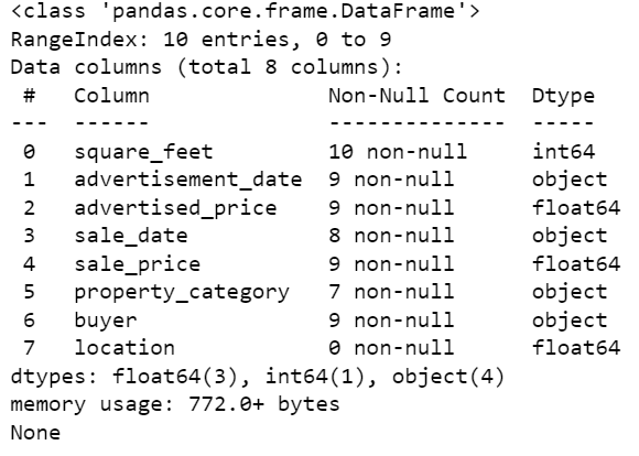
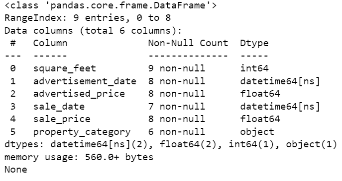
print(df.info())

Here’s the code output.

We can see that only the column square_feet doesn’t have any NULL values, so we’ll somehow have to handle this. Also, the columns advertisement_date, and sale_date are the object data type, even though this should be a date.

The column location is completely empty. Do we need it?

We’ll show you how to handle these issues. We’ll start by learning how to delete unnecessary columns.

There are two columns in the dataset that we don’t need in our data analysis, so we’ll remove them.

The first column is buyer. We don’t need it, as the buyer’s name doesn’t impact the analysis.

We’re using the drop() method with the specified column name. We set the axis to 1 to specify that we want to delete a column. Also, the inplace argument is set to True so that we modify the existing DataFrame, and not create a new DataFrame without the removed column.

df.drop('buyer', axis = 1, inplace = True)

The second column we want to remove is location. While it might be useful to have this information, this is a completely empty column, so let’s just remove it.

We take the same approach as with the first column.

df.drop('location', axis = 1, inplace = True)

Of course, you can remove these two columns simultaneously.

df = df.drop(['buyer', 'location'], axis=1)

Both approaches return the following dataframe.

Duplicate data can occur in your dataset for various reasons and can skew your analysis.

Let’s detect the duplicates in our dataset. Here’s how to do it.

The below code uses the method duplicated() to consider duplicates in the whole dataset. Its default setting is to consider the first occurrence of a value as unique and the subsequent occurrences as duplicates. You can modify this behavior using the keep parameter. For instance, df.duplicated(keep=False) would mark all duplicates as True, including the first occurrence.

# Detecting duplicates
duplicates = df[df.duplicated()]
duplicates

Here’s the output.

The row with index 3 has been marked as duplicate because row 2 with the same values is its first occurrence.

Now we need to remove duplicates, which we do with the following code.

# Detecting duplicates
duplicates = df[df.duplicated()]
duplicates

The drop_duplicates() function considers all columns while identifying duplicates. If you want to consider only certain columns, you can pass them as a list to this function like this: df.drop_duplicates(subset=['column1', 'column2']).

As you can see, the duplicate row has been dropped. However, the indexing stayed the same, with index 3 missing. We’ll tidy this up by resetting indices.

df = df.reset_index(drop=True)

This task is performed by using the reset_index() function. The drop=True argument is used to discard the original index. If you do not include this argument, the old index will be added as a new column in your DataFrame. By setting drop=True, you are telling pandas to forget the old index and reset it to the default integer index.

For practice, try to remove duplicates from this Microsoft dataset.

Sometimes, data types might be incorrectly set. For example, a date column might be interpreted as strings. You need to convert these to their appropriate types.

In our dataset, we’ll do that for the columns advertisement_date and sale_date, as they are shown as the object data type. Also, the date dates are formatted differently across the rows. We need to make it consistent, along with converting it to date.

The easiest way is to use the to_datetime() method. Again, you can do that column by column, as shown below.

When doing that, we set the dayfirst argument to True because some dates start with the day first.

# Converting advertisement_date column to datetime
df['advertisement_date'] = pd.to_datetime(df['advertisement_date'], dayfirst = True) # Converting sale_date column to datetime
df['sale_date'] = pd.to_datetime(df['sale_date'], dayfirst = True)

You can also convert both columns at the same time by using the apply() method with to_datetime().

# Converting advertisement_date and sale_date columns to datetime
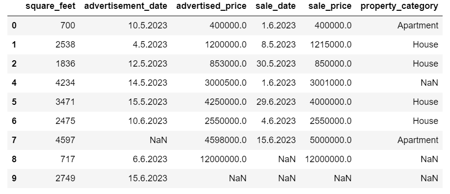
df[['advertisement_date', 'sale_date']] = df[['advertisement_date', 'sale_date']].apply(pd.to_datetime, dayfirst = True)

Both approaches give you the same result.

Now the dates are in a consistent format. We see that not all data has been converted. There’s one NaT value in advertisement_date and two in sale_date. This means the date is missing.

Let’s check if the columns are converted to dates by using the info() method.

# Get a concise summary of the dataframe
print(df.info())

As you can see, both columns are not in datetime64[ns] format.

Now, try to convert the data from TEXT to NUMERIC in this Airbnb dataset.

Real-world datasets often have missing values. Handling missing data is vital, as certain algorithms cannot handle such values.

Our example also has some missing values, so let’s take a look at the two most usual approaches to handling missing data.

Deleting Rows With Missing Values

If the number of rows with missing data is insignificant compared to the total number of observations, you might consider deleting these rows.

In our example, the last row has no values except the square feet and advertisement date. We can’t use such data, so let’s remove this row.

Here’s the code where we indicate the row’s index.

df = df.drop(8)

The DataFrame now looks like this.

The last row has been deleted, and our DataFrame now looks better. However, there are still some missing data which we’ll handle using another approach.

Imputing Missing Values

If you have significant missing data, a better strategy than deleting could be imputation. This process involves filling in missing values based on other data. For numerical data, common imputation methods involve using a measure of central tendency (mean, median, mode).

In our already changed DataFrame, we have NaT (Not a Time) values in the columns advertisement_date and sale_date. We’ll impute these missing values using the mean() method.

The code uses the fillna() method to find and fill the null values with the mean value.

# Imputing values for numerical columns
df['advertisement_date'] = df['advertisement_date'].fillna(df['advertisement_date'].mean())
df['sale_date'] = df['sale_date'].fillna(df['sale_date'].mean())

You can also do the same thing in one line of code. We use the apply() to apply the function defined using lambda. Same as above, this function uses the fillna() and mean() methods to fill in the missing values.

# Imputing values for multiple numerical columns
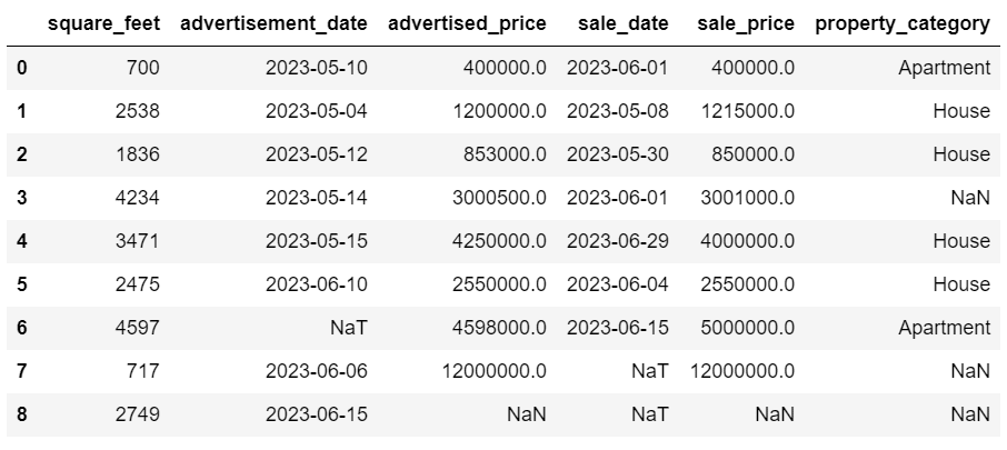
df[['advertisement_date', 'sale_date']] = df[['advertisement_date', 'sale_date']].apply(lambda x: x.fillna(x.mean()))

The output in both cases looks like this.

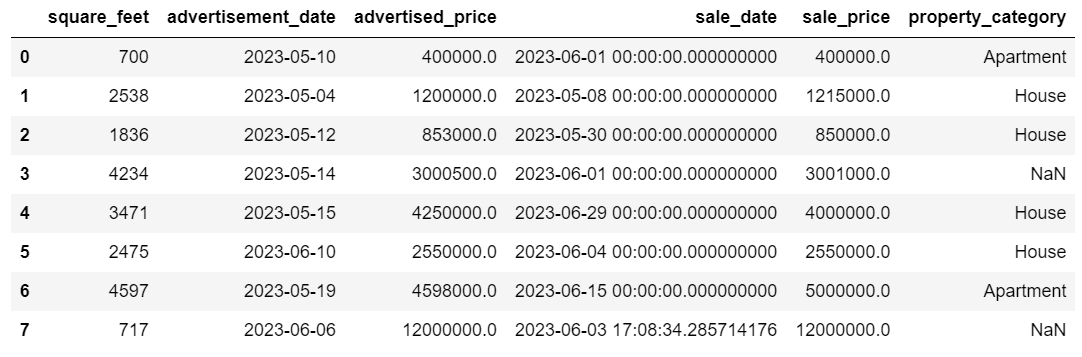
Our sale_date column now has times which we don’t need. Let’s remove them.

We’ll use the strftime() method, which converts the dates to their string representation and a specific format.

df['sale_date'] = df['sale_date'].dt.strftime('%Y-%m-%d')

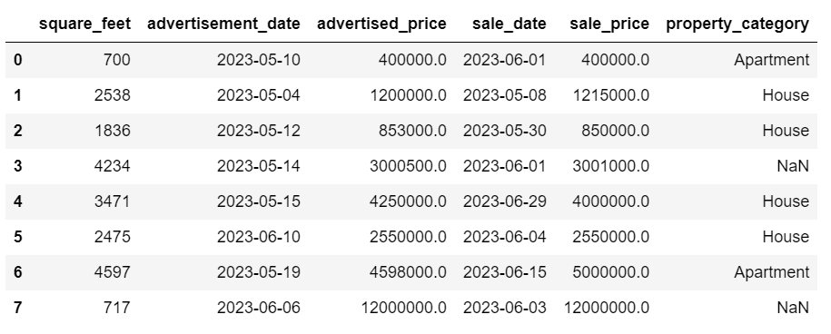
The dates now look all tidy.

If you need to use strftime() on multiple columns, you can again use lambda the following way.

df[['date1_formatted', 'date2_formatted']] = df[['date1', 'date2']].apply(lambda x: x.dt.strftime('%Y-%m-%d'))

Now, let’s see how we can impute missing categorical values.

Categorical data is a type of data that is used to group information with similar characteristics. Each of these groups is a category. Categorical data can take on numerical values (such as "1" indicating "male" and "2" indicating "female"), but those numbers do not have mathematical meaning. You can't add them together, for instance.

Categorical data is typically divided into two categories:

Nominal data: This is when the categories are only labeled and cannot be arranged in any particular order. Examples include gender (male, female), blood type (A, B, AB, O), or color (red, green, blue).

Ordinal data: This is when the categories can be ordered or ranked. While the intervals between the categories are not equally spaced, the order of the categories has a meaning. Examples include rating scales (1 to 5 rating of a movie), an education level (high school, undergraduate, graduate), or stages of cancer (Stage I, Stage II, Stage III).

For imputing missing categorical data, the mode is typically used. In our example, the column property_category is categorical (nominal) data, and there’s data missing in two rows.

Let’s replace the missing values with mode.

# For categorical columns
df['property_category'] = df['property_category'].fillna(df['property_category'].mode()[0])

This code uses the fillna() function to replace all the NaN values in the property_category column. It replaces it with mode.

Additionally, the [0] part is used to extract the first value from this Series. If there are multiple modes, this will select the first one. If there's only one mode, it still works fine.

Here’s the output.

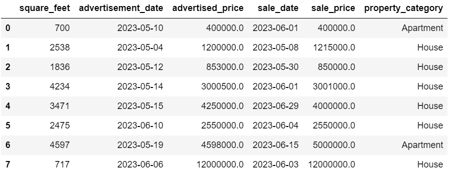
The data now looks pretty good. The only thing that’s remaining is to see if there are outliers.

You can practice dealing with nulls on this Meta interview question, where you’ll have to replace NULLs with zeros.

Outliers are data points in a dataset that are distinctly different from the other observations. They may lie exceptionally far from the other values in the data set, residing outside an overall pattern. They're considered unusual due to their values either being significantly higher or lower compared to the rest of the data.

Outliers can arise due to various reasons such as:

Measurement or input errors
Data corruption
True statistical anomalies

Outliers can significantly impact the results of your data analysis and statistical modeling. They can lead to a skewed distribution, bias, or invalidate the underlying statistical assumptions, distort the estimated model fit, reduce the predictive accuracy of predictive models, and lead to incorrect conclusions.

Some commonly used methods to detect outliers are Z-score, IQR (Interquartile Range), box plots, scatter plots, and data visualization techniques. In some advanced cases, machine learning methods are used as well.

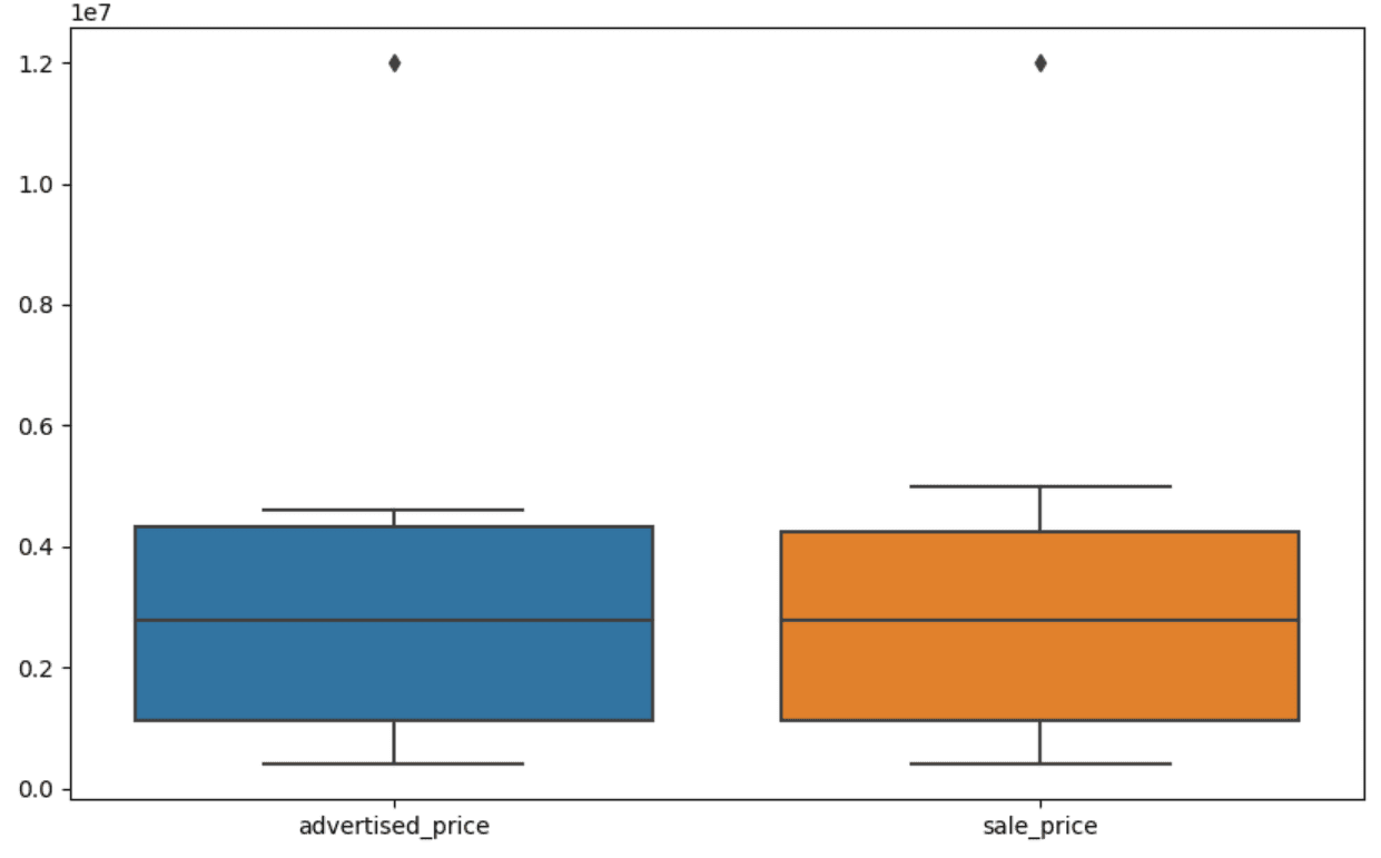
Visualizing data can help identify outliers. Seaborn's boxplot is handy for this.

plt.figure(figsize=(10, 6))
sns.boxplot(data=df[['advertised_price', 'sale_price']])

We use the plt.figure() to set the width and height of the figure in inches.

Then we create the boxplot for the columns advertised_price and sale_price, which looks like this.

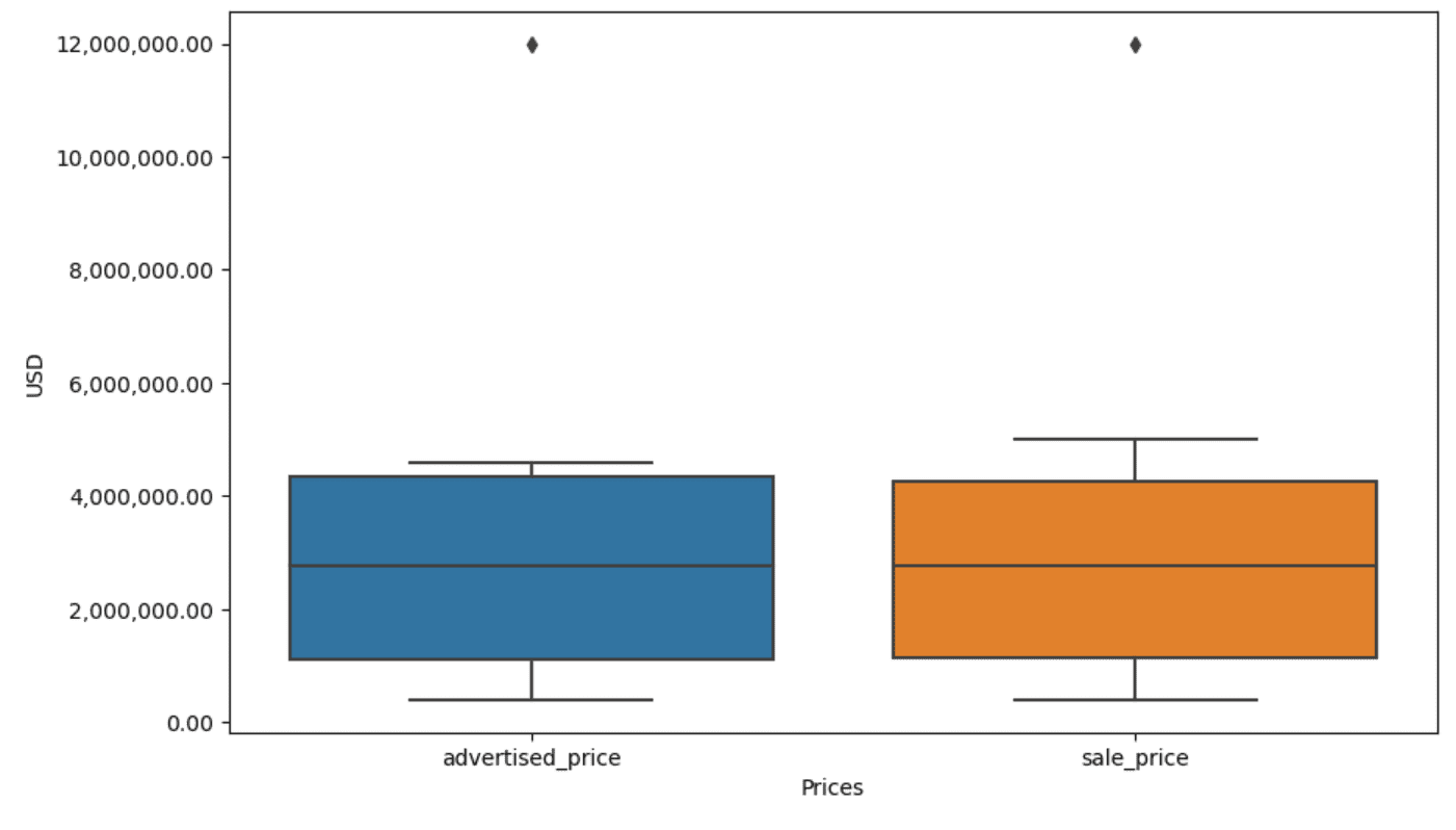
The plot can be improved for easier use by adding this to the above code.

plt.xlabel('Prices')
plt.ylabel('USD')
plt.ticklabel_format(style='plain', axis='y')
formatter = ticker.FuncFormatter(lambda x, p: format(x, ',.2f'))
plt.gca().yaxis.set_major_formatter(formatter)

We use the above code to set the labels for both axes. We also notice that the values on the y-axis are in the scientific notation, and we can’t use that for the price values. So we change this to plain style using the plt.ticklabel_format() function.

Then we create the formatter that will show the values on the y-axis with commas as thousand separators and decimal dots. The last code line applies this to the axis.

The output now looks like this.

Now, how do we identify and remove the outlier?

One of the ways is to use the IQR method.

IQR, or Interquartile Range, is a statistical method used to measure variability by dividing a data set into quartiles. Quartiles divide a rank-ordered data set into four equal parts, and values within the range of the first quartile (25th percentile) and the third quartile (75th percentile) make up the interquartile range.

The interquartile range is used to identify outliers in the data. Here's how it works:

First, calculate the first quartile (Q1), the third quartile (Q3), and then determine the IQR. The IQR is computed as Q3 - Q1.
Any value below Q1 - 1.5IQR or above Q3 + 1.5IQR is considered an outlier.

On our boxplot, the box actually represents the IQR. The line inside the box is the median (or second quartile). The 'whiskers' of the boxplot represent the range within 1.5*IQR from Q1 and Q3.

Any data points outside these whiskers can be considered outliers. In our case, it’s the value of $12,000,000. If you look at the boxplot, you’ll see how clearly this is represented, which shows why data visualization is important in detecting outliers.

Now, let’s remove the outliers by using the IQR method in Python code. First, we’ll remove the advertised price outliers.

Q1 = df['advertised_price'].quantile(0.25)
Q3 = df['advertised_price'].quantile(0.75)
IQR = Q3 - Q1
df = df[~((df['advertised_price'] (Q1 - 1.5 * IQR)) |(df['advertised_price'] > (Q3 + 1.5 * IQR)))]

We first calculate the first quartile (or the 25th percentile) using the quantile() function. We do the same for the third quartile or the 75th percentile.

They show the values below which 25% and 75% of the data fall, respectively.

Then we calculate the difference between the quartiles. Everything so far is just translating the IQR steps into Python code.

As a final step, we remove the outliers. In other words, all data less than Q1 - 1.5 * IQR or more than Q3 + 1.5 * IQR.

The '~' operator negates the condition, so we are left with only the data that are not outliers.

Then we can do the same with the sale price.

Q1 = df['sale_price'].quantile(0.25)
Q3 = df['sale_price'].quantile(0.75)
IQR = Q3 - Q1
df = df[~((df['sale_price'] (Q1 - 1.5 * IQR)) |(df['sale_price'] > (Q3 + 1.5 * IQR)))]

Of course, you can do it in a more succinct way using the for loop.

for column in ['advertised_price', 'sale_price']: Q1 = df[column].quantile(0.25) Q3 = df[column].quantile(0.75) IQR = Q3 - Q1 df = df[~((df[column] (Q1 - 1.5 * IQR)) |(df[column] > (Q3 + 1.5 * IQR)))]

The loop iterates of the two columns. For each column, it calculates the IQR and then removes the rows in the DataFrame.

Please note that this operation is done sequentially, first for advertised_price and then for sale_price. As a result, the DataFrame is modified in-place for each column, and rows can be removed due to being an outlier in either column. Therefore, this operation might result in fewer rows than if outliers for advertised_price and sale_price were removed independently and the results were combined afterward.

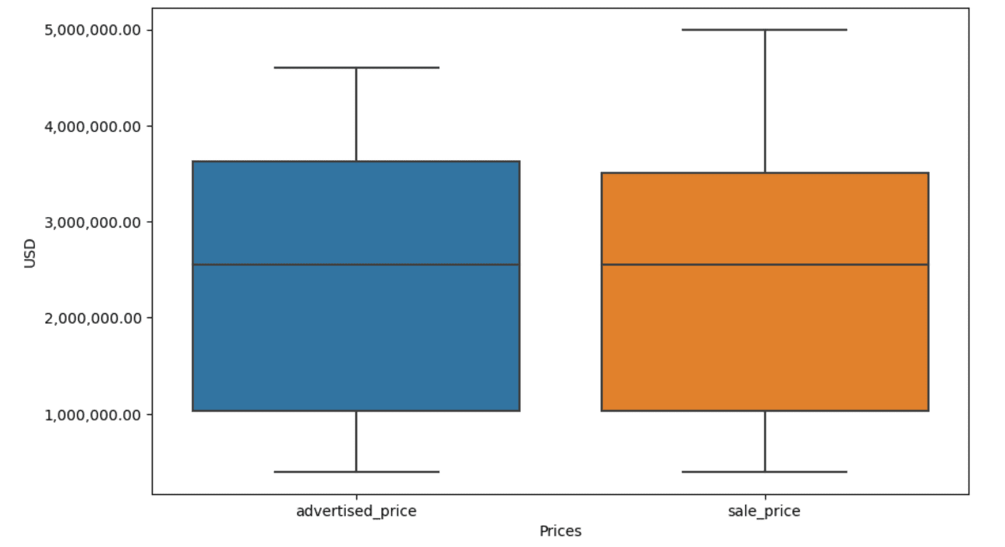
In our example, the output will be the same in both cases. To see how the box plot changed, we need to plot it again using the same code as earlier.

plt.figure(figsize=(10, 6))
sns.boxplot(data=df[['advertised_price', 'sale_price']])
plt.xlabel('Prices')
plt.ylabel('USD')
plt.ticklabel_format(style='plain', axis='y')
formatter = ticker.FuncFormatter(lambda x, p: format(x, ',.2f'))
plt.gca().yaxis.set_major_formatter(formatter)

Here’s the output.

You can practice calculating percentiles in Python by solving the General Assembly interview question.

Data cleaning is a crucial step in the data analysis process. Though it can be time-consuming, it's essential to ensure the accuracy of your findings.

Fortunately, Python's rich ecosystem of libraries makes this process more manageable. We learned how to remove unnecessary rows and columns, reformat data, and deal with missing values and outliers. These are the usual steps that have to be performed on most any data. However, you’ll also sometimes need to combine two columns into one, verify the existing data, assign labels to it, or get rid of the white spaces.

All this is data cleaning, as it allows you to turn messy, real-world data into a well-structured dataset that you can analyze with confidence. Just compare the dataset we started with to the one we ended up with.

If you don’t see the satisfaction in this result and the clean data doesn’t make you strangely excited, what in the world are you doing in data science!?

Nate Rosidi is a data scientist and in product strategy. He's also an adjunct professor teaching analytics, and is the founder of StrataScratch, a platform helping data scientists prepare for their interviews with real interview questions from top companies. Connect with him on Twitter: StrataScratch or LinkedIn.