图片作者
When you are getting started with machine learning, logistic regression is one of the first algorithms you’ll add to your toolbox. It’s a simple and robust algorithm, commonly used for binary classification tasks.
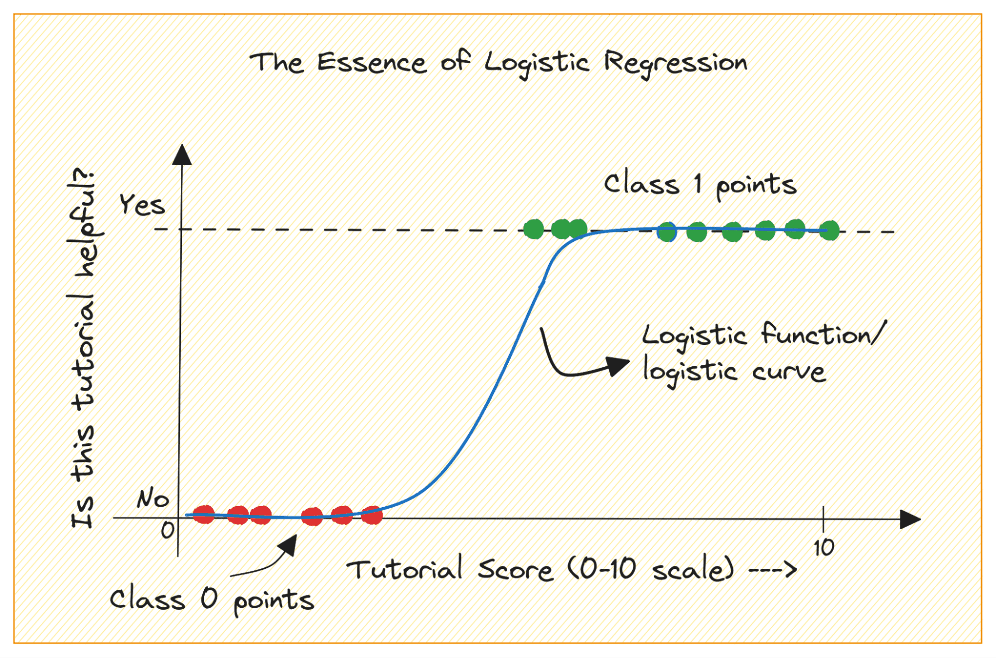
考虑类别 0 和 1 的二元分类问题。逻辑回归将逻辑或 sigmoid 函数拟合到输入数据,并预测查询数据点属于类别 1 的概率。有趣,是吗?
在本教程中,我们将从头开始学习逻辑回归,包括:
- 逻辑(或 sigmoid)函数
- 我们如何从线性回归转向逻辑回归
- 逻辑回归的工作原理
最后,我们将构建一个简单的逻辑回归模型 对电离层雷达回波进行分类.
Before we learn more about logistic regression, let’s review how the logistic function works. The logistic (or sigmoid function) is given by:

当您绘制 sigmoid 函数时,它看起来像这样:
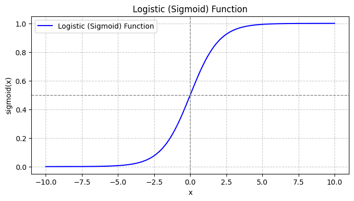
从剧情中我们可以看出:
- 当 x = 0 时,σ(x) 的值为 0.5。
- 当 x 接近 +∞ 时,σ(x) 接近 1。
- 当 x 接近 -∞ 时,σ(x) 接近 0。
因此,对于所有实数输入,sigmoid 函数会将它们压缩为 [0, 1] 范围内的值。
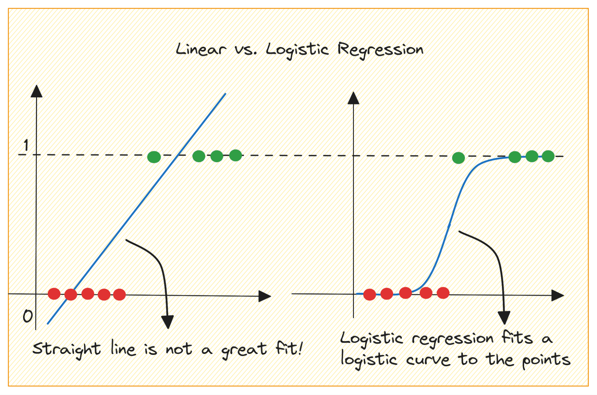
Let’s first discuss why we cannot use linear regression for a binary classification problem.
在二元分类问题中,输出是分类标签(0 或 1)。由于线性回归预测的连续值输出可能小于 0 或大于 1,因此它对于当前的问题没有意义。
此外,当输出标签属于两个类别之一时,直线可能不是最佳拟合。
图片作者
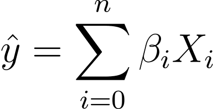
那么我们如何从线性回归转向逻辑回归呢?在线性回归中,预测输出由下式给出:

其中 βs 是系数,X_is 是预测变量(或特征)。
不失一般性,我们假设 X_0 = 1:

所以我们可以有一个更简洁的表达方式:
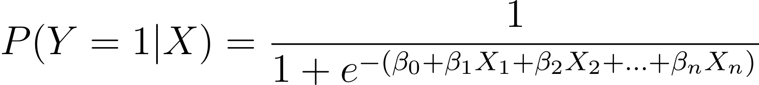
在逻辑回归中,我们需要[0,1]区间内的预测概率p_i。我们知道逻辑函数会压缩输入,使其呈现 [0,1] 区间内的值。
因此,将此表达式代入逻辑函数中,我们的预测概率为:

那么我们如何找到给定数据集的最佳拟合逻辑曲线呢?为了回答这个问题,让我们了解最大似然估计。
最大似然估计(MLE) is used to estimate the parameters of the logistic regression model by maximizing the likelihood function. Let’s break down the process of MLE in logistic regression and how the cost function is formulated for optimization using gradient descent.
分解最大似然估计
正如所讨论的,我们将二元结果发生的概率建模为一个或多个预测变量(或特征)的函数:
Here, the βs are the model parameters or coefficients. X_1, X_2,…, X_n are the predictor variables.
MLE 旨在找到使观测数据的可能性最大化的 β 值。似然函数表示为 L(β),表示在逻辑回归模型下观察给定预测变量值的给定结果的概率。
制定对数似然函数
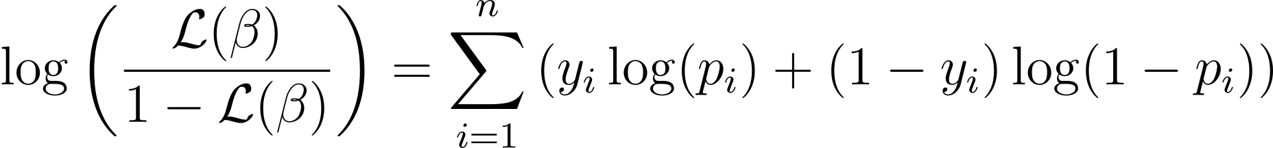
To simplify the optimization process, it’s common to work with the log-likelihood function. Because it transforms products of probabilities into sums of log probabilities.
逻辑回归的对数似然函数由下式给出:
Now that we know the essence of log-likelihood, let’s proceed to formulate the cost function for logistic regression and subsequently gradient descent for finding the best model parameters
逻辑回归的成本函数
为了优化逻辑回归模型,我们需要最大化对数似然。因此,我们可以使用负对数似然作为成本函数,在训练期间最小化。负对数似然,通常称为逻辑损失,定义为:
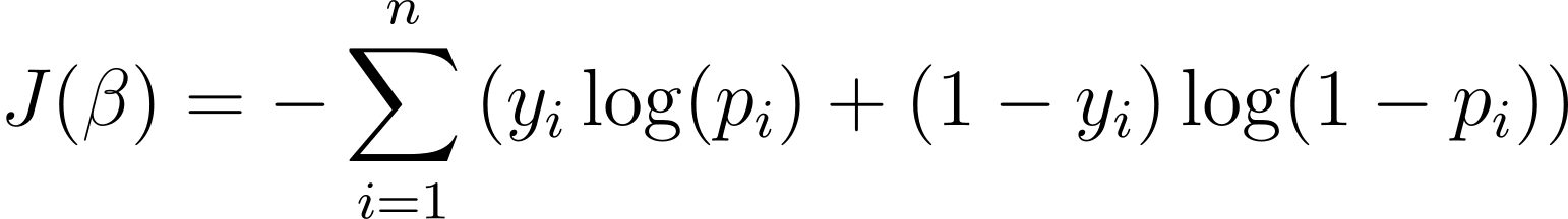
因此,学习算法的目标是找到 ? 的值。最小化这个成本函数。梯度下降是一种常用的优化算法,用于寻找该成本函数的最小值。
逻辑回归中的梯度下降
梯度下降 是一种迭代优化算法,以与成本函数相对于 β 的梯度相反的方向更新模型参数 β。使用梯度下降的逻辑回归在步骤t+1的更新规则如下:
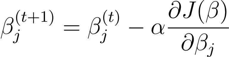
其中 α 是学习率。
偏导数可以使用链式法则计算。梯度下降迭代更新参数,直到收敛,旨在最大限度地减少逻辑损失。当它收敛时,它会找到使观测数据的可能性最大化的 β 的最佳值。
现在您已经了解了逻辑回归的工作原理,接下来让我们使用 scikit-learn 库构建一个预测模型。
我们将使用 来自 UCI 机器学习存储库的电离层数据集 对于本教程。该数据集包含 34 个数字特征。输出是二进制的,“好”或“坏”之一(用“g”或“b”表示)。输出标签“良好”是指雷达回波已检测到电离层中的某些结构。
第 1 步 – 加载数据集
首先,下载数据集并将其读入 pandas 数据框:
import pandas as pd
import urllib

url = "https://archive.ics.uci.edu/ml/machine-learning-databases/ionosphere/iphere.data"
data = urllib.request.urlopen(url)
df = pd.read_csv(data, header=None)
第 2 步 – 探索数据集
Let’s take a look at the first few rows of the dataframe:
# Display the first few rows of the DataFrame
df.head()
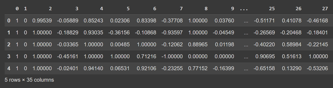
df.head() 的截断输出
Let’s get some information about the dataset: the number of non-null values and the data types of each of the columns:
# Get information about the dataset
print(df.info())
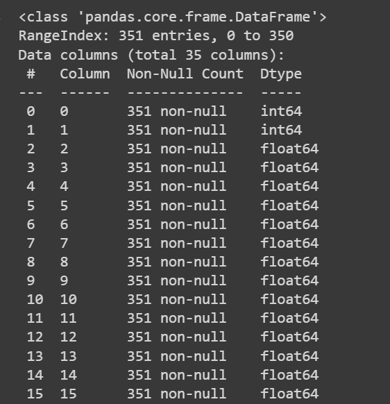 df.info() 的截断输出
因为我们拥有所有数字特征,所以我们还可以使用以下方法获得一些描述性统计数据: describe() 数据框上的方法:
# Get descriptive statistics of the dataset
print(df.describe())
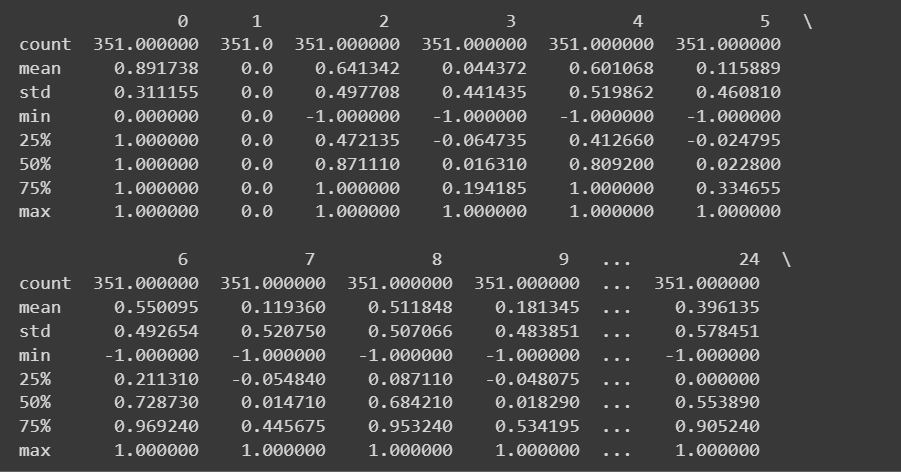
df.describe() 的截断输出
列名称当前为 0 到 34 — 包括标签。由于数据集不提供列的描述性名称,因此如果您希望重命名数据框的列,它只会将它们引用为 attribute_1 到 attribute_34,如下所示:
column_names = [
"attribute_1", "attribute_2", "attribute_3", "attribute_4", "attribute_5",
"attribute_6", "attribute_7", "attribute_8", "attribute_9", "attribute_10",
"attribute_11", "attribute_12", "attribute_13", "attribute_14", "attribute_15",
"attribute_16", "attribute_17", "attribute_18", "attribute_19", "attribute_20",
"attribute_21", "attribute_22", "attribute_23", "attribute_24", "attribute_25",
"attribute_26", "attribute_27", "attribute_28", "attribute_29", "attribute_30",
"attribute_31", "attribute_32", "attribute_33", "attribute_34", "class_label"
]
df.columns = column_names
注意:此步骤完全是可选的。如果您愿意,可以继续使用默认列名称。
# Display the first few rows of the DataFrame
df.head()
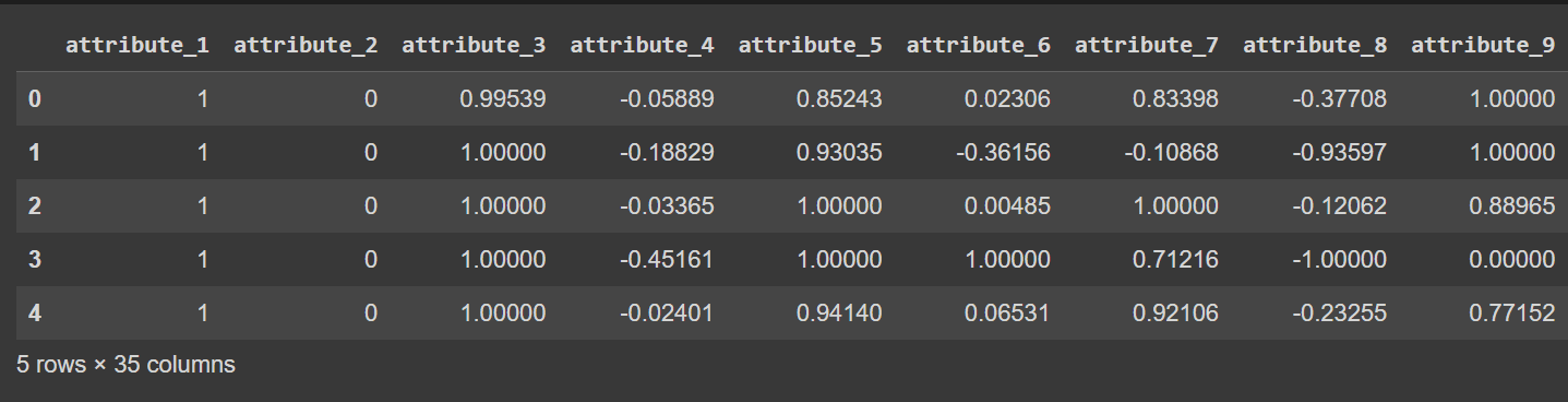
df.head() 的输出被截断[重命名列之后]
步骤 3 – 重命名类标签并可视化类分布
因为输出类标签是 'g' 和 'b',所以我们需要将它们分别映射到 1 和 0 。你可以使用 map() or replace():
# Convert the class labels from 'g' and 'b' to 1 and 0, respectively
df["class_label"] = df["class_label"].replace({'g': 1, 'b': 0})
我们还可以可视化类标签的分布:
import matplotlib.pyplot as plt

# Count the number of data points in each class
class_counts = df['class_label'].value_counts()

# Create a bar plot to visualize the class distribution
plt.bar(class_counts.index, class_counts.values)
plt.xlabel('Class Label')
plt.ylabel('Count')
plt.xticks(class_counts.index)
plt.title('Class Distribution')
plt.show()
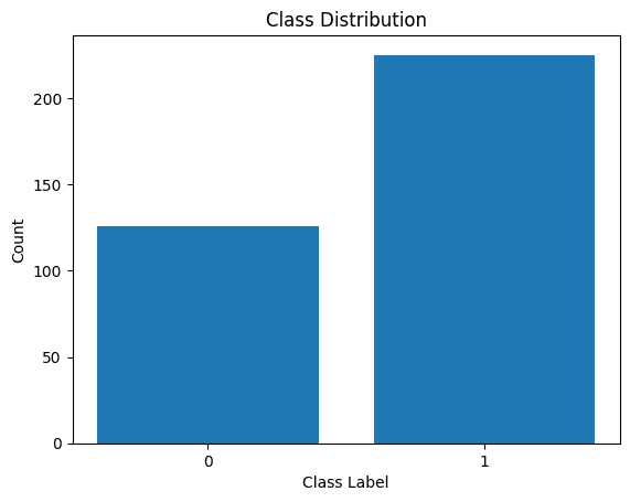
类别标签的分布
我们看到分配不平衡。属于类别 1 的记录多于属于类别 0 的记录。我们将在构建逻辑回归模型时处理这种类别不平衡问题。
步骤 5 – 预处理数据集
让我们像这样收集特征和输出标签:
X = df.drop('class_label', axis=1)  # Input features
y = df['class_label']               # Target variable
将数据集分为训练集和测试集后,我们需要对数据集进行预处理。
当有许多数字特征时(每个特征的尺度可能不同),我们需要对数字特征进行预处理。一种常见的方法是对它们进行变换,使它们遵循均值为零、单位方差为零的分布。
StandardScaler scikit-learn 的预处理模块帮助我们实现了这一点。
from sklearn.preprocessing import StandardScaler
from sklearn.model_selection import train_test_split

# Split the dataset into training and testing sets
X_train, X_test, y_train, y_test = train_test_split(X, y, test_size=0.2, random_state=42)

# Get the indices of the numerical features
numerical_feature_indices = list(range(34))  # Assuming the numerical features are in columns 0 to 33

# Initialize the StandardScaler
scaler = StandardScaler()

# Normalize the numerical features in the training set
X_train.iloc[:, numerical_feature_indices] = scaler.fit_transform(X_train.iloc[:, numerical_feature_indices])

# Normalize the numerical features in the test set using the trained scaler from the training set
X_test.iloc[:, numerical_feature_indices] = scaler.transform(X_test.iloc[:, numerical_feature_indices])
第 6 步 – 构建逻辑回归模型
现在我们可以实例化一个逻辑回归分类器。这 LogisticRegression 类是 scikit-learn 的 Linear_model 模块的一部分。
请注意,我们已经设置了 class_weight 参数为“平衡”。这将帮助我们解决类别不平衡的问题。通过为每个类别分配权重,与类别中的记录数量成反比。
实例化该类后,我们可以将模型拟合到训练数据集:
from sklearn.linear_model import LogisticRegression

model = LogisticRegression(class_weight='balanced')
model.fit(X_train, y_train)
步骤 7 – 评估逻辑回归模型
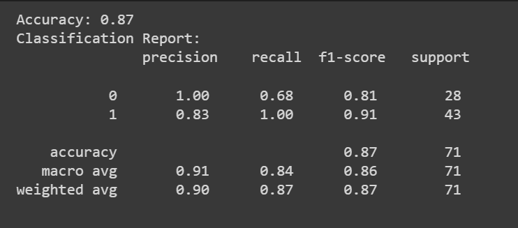
您可以拨打 predict() 方法来获得模型的预测。
除了准确率分数之外,我们还可以获得包含精度、召回率和 F1 分数等指标的分类报告。
from sklearn.metrics import accuracy_score, classification_report

y_pred = model.predict(X_test)
accuracy = accuracy_score(y_test, y_pred)
print(f"Accuracy: {accuracy:.2f}")

classification_rep = classification_report(y_test, y_pred)
print("Classification Report:n", classification_rep)
恭喜,您已经编写了第一个逻辑回归模型!
在本教程中,我们详细了解了逻辑回归:从理论和数学到编码逻辑回归分类器。
下一步,尝试为您选择的合适数据集构建逻辑回归模型。
电离层数据集已获得许可 知识共享署名 4.0 国际 (CC BY 4.0)许可证:
Sigillito,V.、Wing,S.、Hutton,L. 和 Baker,K.(1989)。电离层。 UCI 机器学习存储库。 https://doi.org/10.24432/C5W01B。
巴拉普里亚 C 是来自印度的开发人员和技术作家。 她喜欢在数学、编程、数据科学和内容创作的交叉领域工作。 她的兴趣和专长领域包括 DevOps、数据科学和自然语言处理。 她喜欢阅读、写作、编码和咖啡! 目前,她致力于通过编写教程、操作指南、评论文章等方式学习并与开发人员社区分享她的知识。
- SEO 支持的内容和 PR 分发。 今天得到放大。
- PlatoData.Network 垂直生成人工智能。 赋予自己力量。 访问这里。
- 柏拉图爱流。 Web3 智能。 知识放大。 访问这里。
- 柏拉图ESG。 碳, 清洁科技, 能源, 环境, 太阳能, 废物管理。 访问这里。
- 柏拉图健康。 生物技术和临床试验情报。 访问这里。
- Sumber: https://www.kdnuggets.com/building-predictive-models-logistic-regression-in-python?utm_source=rss&utm_medium=rss&utm_campaign=building-predictive-models-logistic-regression-in-python
- :是
- :不是
- $UP
- 1
- 10
- 11
- 13
- 20
- 33
- 7
- 9
- a
- 关于
- 账号管理
- 加
- 增加
- 后
- 目标
- 算法
- 算法
- 所有类型
- 还
- an
- 和
- 回答
- 方法
- 保健
- 地区
- AS
- 承担
- At
- 创作
- b
- 面包师傅
- 均衡
- 酒吧
- BE
- 因为
- 属于
- 最佳
- 午休
- 建立
- 建筑物
- by
- 呼叫
- CAN
- 不能
- 类别
- 链
- 选择
- 程
- 类
- 分类
- 编码
- 编码
- 收集
- 柱
- 列
- 相当常见
- 常用
- 共享
- 社体的一部分
- 包含
- 简洁
- 内容
- 内容创造
- 兑换
- 价格
- 覆盖
- 创建信息图
- 创建
- 目前
- 曲线
- data
- 数据点
- 数据科学
- 数据集
- 默认
- 定义
- 衍生工具
- 细节
- 检测
- 开发商
- DevOps的
- 不同
- 方向
- 讨论
- 讨论
- 屏 显:
- 分配
- do
- 不
- 向下
- 下载
- ,我们将参加
- 每
- 本质
- 评估
- 评估
- 专门知识
- 探索
- 表达
- 特征
- 少数
- 找到最适合您的地方
- 寻找
- 发现
- 姓氏:
- 适合
- 遵循
- 如下
- 针对
- FRAME
- 止
- 功能
- 得到
- 越来越
- 特定
- Go
- 目标
- 谷歌
- 更大的
- 陆运
- 指南
- 手
- 处理
- 有
- 帮助
- 帮助
- 这里
- 创新中心
- HTTPS
- ICS
- if
- 失调
- 进口
- in
- 包括
- 指数
- 印度
- 指数
- 信息
- 输入
- 输入
- 兴趣
- 有趣
- 路口
- 成
- IT
- 只是
- 掘金队
- 知道
- 知识
- 标签
- 标签
- 语言
- 学习用品
- 知道
- 学习
- 减
- 让
- 自学资料库
- 执照
- 行货
- 喜欢
- 可能性
- 喜欢
- Line
- 装载
- 日志
- 看
- 看起来像
- 离
- 机
- 机器学习
- 使
- 许多
- 地图
- 数学
- matplotlib
- 生产力
- 最大化
- 最多
- 可能..
- 意味着
- 方法
- 指标
- 大幅减低
- 最低限度
- 模型
- 模型
- 模块
- 更多
- 移动
- 名称
- 自然
- 自然语言
- 自然语言处理
- 需求
- 负
- 下页
- 数
- 观察
- of
- 经常
- on
- 一
- 检讨
- 相反
- 最佳
- 优化
- 优化
- or
- 成果
- 结果
- 产量
- 输出
- 大熊猫
- 参数
- 参数
- 部分
- 件
- 柏拉图
- 柏拉图数据智能
- 柏拉图数据
- 点
- 点
- 可能
- 平台精度
- 都曾预测
- 预测
- 预测
- 预报器
- 预测
- 比较喜欢
- 可能性
- 市场问题
- 继续
- 过程
- 处理
- 核心产品
- 代码编程
- 提供
- 纯粹
- 蟒蛇
- 雷达
- 范围
- 率
- 阅读
- 阅读
- 真实
- 记录
- 简称
- 指
- 回归
- 报告
- 知识库
- 代表
- 请求
- 尊重
- 分别
- 回报
- 检讨
- 健壮
- 第
- s
- 科学
- scikit学习
- 得分了
- 看到
- 感
- 集
- 套数
- 共享
- 她
- 如图
- 简易
- 简化
- So
- 一些
- 分裂
- 开始
- 统计
- 步
- 直
- 结构体
- 后来
- 这样
- 合适的
- 总和
- 采取
- 需要
- 目标
- 任务
- 文案
- test
- 测试
- 比
- 这
- 他们
- 理论
- 那里。
- 因此
- 他们
- Free Introduction
- 通过
- 至
- 工具箱
- 培训
- 熟练
- 产品培训
- 改造
- 变换
- 尝试
- 教程
- 教程
- 二
- 类型
- 下
- 理解
- 单元
- 更新
- 最新动态
- 网址
- us
- 美国账户
- 使用
- 用过的
- 运用
- 折扣值
- 价值观
- 想像
- we
- ,尤其是
- 这
- 为什么
- 维基百科上的数据
- 将
- 翼
- 工作
- 加工
- 合作
- 将
- 作家
- 写作
- X
- 含
- 您
- 您一站式解决方案
- 和风网
- 零