[Image by Author]
The concept of “feature importance” is widely used in machine learning as the most basic type of model explainability. For example, it is used in Recursive Feature Elimination (RFE), to iteratively drop the least important feature of the model.
However, there is a misconception about it.
The fact that a feature is important doesn’t imply that it is beneficial for the model!
Indeed, when we say that a feature is important, this simply means that the feature brings a high contribution to the predictions made by the model. But we should consider that such contribution may be wrong.
Take a simple example: a data scientist accidentally forgets the Customer ID between its model’s features. The model uses Customer ID as a highly predictive feature. As a consequence, this feature will have a high feature importance even if it is actually worsening the model, because it cannot work well on unseen data.
To make things clearer, we will need to make a distinction between two concepts:
- Prediction Contribution: what part of the predictions is due to the feature; this is equivalent to feature importance.
- Error Contribution: what part of the prediction errors is due to the presence of the feature in the model.
In this article, we will see how to calculate these quantities and how to use them to get valuable insights about a predictive model (and to improve it).
Note: this article is focused on the regression case. If you are more interested in the classification case, you can read “Which features are harmful for your classification model?”
Suppose we built a model to predict the income of people based on their job, age, and nationality. Now we use the model to make predictions on three people.
Thus, we have the ground truth, the model prediction, and the resulting error:
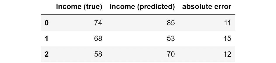
Ground truth, model prediction, and absolute error (in thousands of $). [Image by Author]
When we have a predictive model, we can always decompose the model predictions into the contributions brought by the single features. This can be done through SHAP values (if you don’t know about how SHAP values work, you can read my article: SHAP Values Explained Exactly How You Wished Someone Explained to You).
So, let’s say these are the SHAP values relative to our model for the three individuals.

SHAP values for our model’s predictions (in thousands of $). [Image by Author]
The main property of SHAP values is that they are additive. This means that — by taking the sum of each row — we will obtain our model’s prediction for that individual. For instance, if we take the second row: 72k $ +3k $ -22k $ = 53k $, which is exactly the model’s prediction for the second individual.
Now, SHAP values are a good indicator of how important a feature is for our predictions. Indeed, the higher the (absolute) SHAP value, the more influential the feature for the prediction about that specific individual. Note that I am talking about absolute SHAP values because the sign here doesn’t matter: a feature is equally important if it pushes the prediction up or down.
Therefore, the Prediction Contribution of a feature is equal to the mean of the absolute SHAP values of that feature. If you have the SHAP values stored in a Pandas dataframe, this is as simple as:
prediction_contribution = shap_values.abs().mean()In our example, this is the result:

Prediction Contribution. [Image by Author]
As you can see, job is clearly the most important feature since, on average, it accounts for 71.67k $ of the final prediction. Nationality and age are respectively the second and the third most relevant feature.
However, the fact that a given feature accounts for a relevant part of the final prediction doesn’t tell anything about the feature’s performance. To consider also this aspect, we will need to compute the “Error Contribution”.
Let’s say that we want to answer the following question: “What predictions would the model make if it didn’t have the feature job?” SHAP values allow us to answer this question. In fact, since they are additive, it’s enough to subtract the SHAP values relative to the feature job from the predictions made by the model.
Of course, we can repeat this procedure for each feature. In Pandas:
y_pred_wo_feature = shap_values.apply(lambda feature: y_pred - feature)This is the outcome:

Predictions that we would obtain if we removed the respective feature. [Image by Author]
This means that, if we didn’t have the feature job, then the model would predict 20k $ for the first individual, -19k $ for the second one, and -8k $ for the third one. Instead, if we didn’t have the feature age, the model would predict 73k $ for the first individual, 50k $ for the second one, and so on.
As you can see, the predictions for each individual vary a lot if we removed different features. As a consequence, also the prediction errors would be very different. We can easily compute them:
abs_error_wo_feature = y_pred_wo_feature.apply(lambda feature: (y_true - feature).abs())The result is the following:

Absolute errors that we would obtain if we removed the respective feature. [Image by Author]
These are the errors that we would obtain if we removed the respective feature. Intuitively, if the error is small, then removing the feature is not a problem — or it’s even beneficial — for the model. If the error is high, then removing the feature is not a good idea.
But we can do more than this. Indeed, we can compute the difference between the errors of the full model and the errors we would obtain without the feature:
error_diff = abs_error_wo_feature.apply(lambda feature: abs_error - feature)Which is:

Difference between the errors of the model and the errors we would have without the feature. [Image by Author]
If this number is:
- negative, then the presence of the feature leads to a reduction in the prediction error, so the feature works well for that observation!
- positive, then the presence of the feature leads to an increase in the prediction error, so the feature is bad for that observation.
We can compute “Error Contribution” as the mean of these values, for each feature. In Pandas:
error_contribution = error_diff.mean()This is the outcome:

Error Contribution. [Image by Author]
If this value is positive, then it means that, on average, the presence of the feature in the model leads to a higher error. Thus, without that feature, the prediction would have been generally better. In other words, the feature is making more harm than good!
On the contrary, the more negative this value, the more beneficial the feature is for the predictions since its presence leads to smaller errors.
Let’s try to use these concepts on a real dataset.
Hereafter, I will use a dataset taken from Pycaret (a Python library under MIT license). The dataset is called “Gold” and it contains time series of financial data.
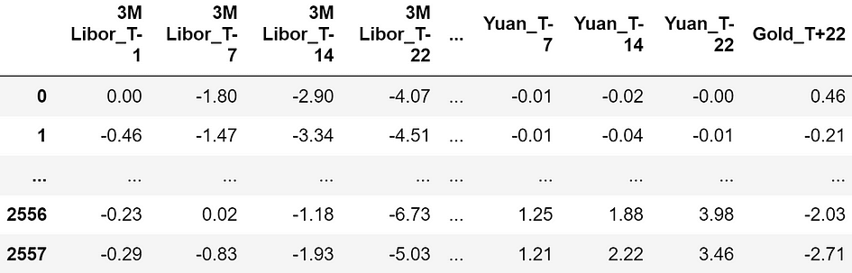
Dataset sample. The features are all expressed in percentage, so -4.07 means a return of -4.07%. [Image by Author]
The features consist in the returns of financial assets respectively 22, 14, 7, and 1 days before the observation moment (“T-22”, “T-14”, “T-7”, “T-1”). Here is the exhaustive list of all the financial assets used as predictive features:
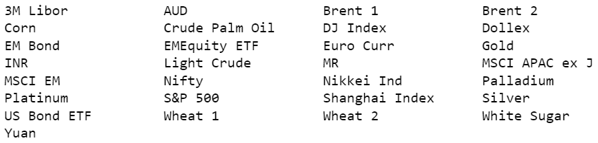
List of the available assets. Each asset is observed at time -22, -14, -7, and -1. [Image by Author]
In total, we have 120 features.
The goal is to predict the Gold price (return) 22 days ahead in time (“Gold_T+22”). Let’s take a look at the target variable.
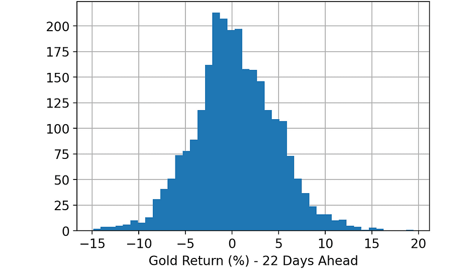
Histogram of the variable. [Image by Author]
Once I loaded the dataset, these are the steps I carried out:
- Split the full dataset randomly: 33% of the rows in the training dataset, another 33% in the validation dataset, and the remaining 33% in the test dataset.
- Train a LightGBM Regressor on the training dataset.
- Make predictions on training, validation, and test datasets, using the model trained at the previous step.
- Compute SHAP values of training, validation, and test datasets, using the Python library “shap”.
- Compute the Prediction Contribution and the Error Contribution of each feature on each dataset (training, validation, and test), using the code we have seen in the previous paragraph.
Let’s compare the Error Contribution and the Prediction Contribution in the training dataset. We will use a scatter plot, so the dots identify the 120 features of the model.
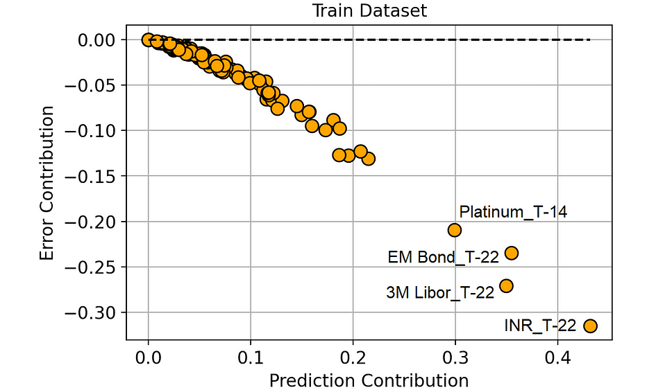
Prediction Contribution vs. Error Contribution (on the Training dataset). [Image by Author]
There is a highly negative correlation between Prediction Contribution and Error Contribution in the training set.
And this makes sense: since the model learns on the training dataset, it tends to attribute high importance (i.e. high Prediction Contribution) to those features that lead to a great reduction in the prediction error (i.e. highly negative Error Contribution).
But this doesn’t add much to our knowledge, right?
Indeed, what really matters to us is the validation dataset. The validation dataset is in fact the best proxy we can have about how our features will behave on new data. So, let’s make the same comparison on the validation set.
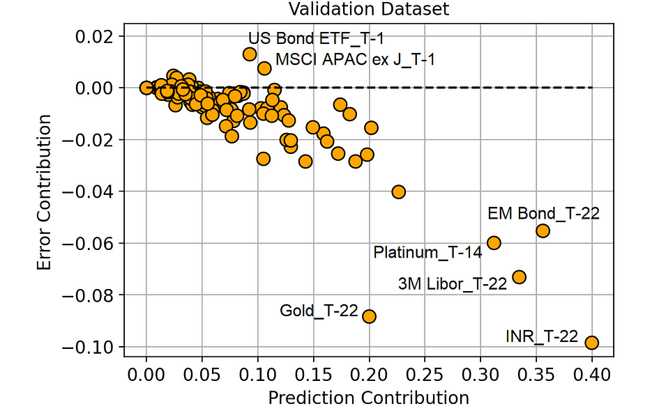
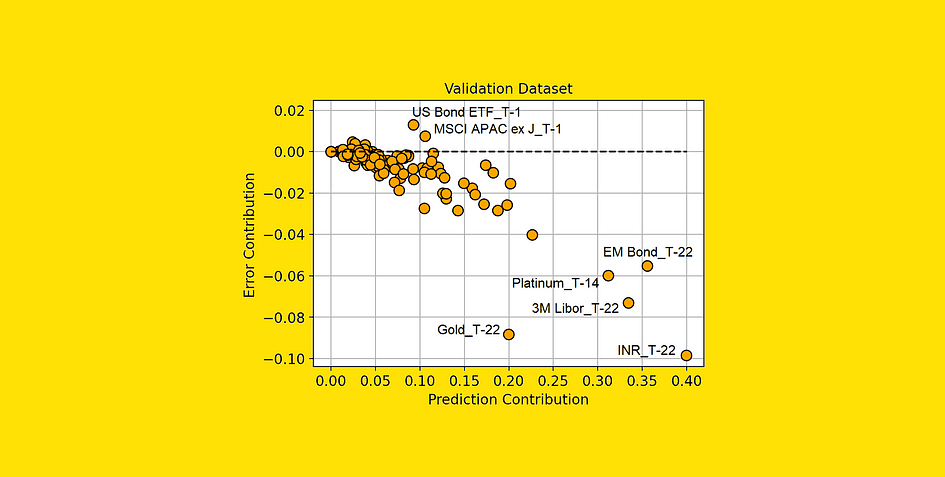
Prediction Contribution vs. Error Contribution (on the Validation dataset). [Image by Author]
From this plot, we can extract some much more interesting information.
The features in the lower right part of the plot are those to which our model is correctly assigning high importance since they actually bring a reduction in the prediction error.
Also, note that “Gold_T-22” (the return of gold 22 days before the observation period) is working really well compared to the importance that the model is attributing to it. This means that this feature is possibly underfitting. And this piece of information is particularly interesting since gold is the asset we are trying to predict (“Gold_T+22”).
On the other hand, the features that have an Error Contribution above 0 are making our predictions worse. For instance, “US Bond ETF_T-1” on average changes the model prediction by 0.092% (Prediction Contribution), but it leads the model to make a prediction on average 0.013% (Error Contribution) worse than it would have been without that feature.
We may suppose that all the features with a high Error Contribution (compared to their Prediction Contribution) are probably overfitting or, in general, they have different behavior in the training set and in the validation set.
Let’s see which features have the largest Error Contribution.
Features sorted by decreasing Error Contribution. [Image by Author]
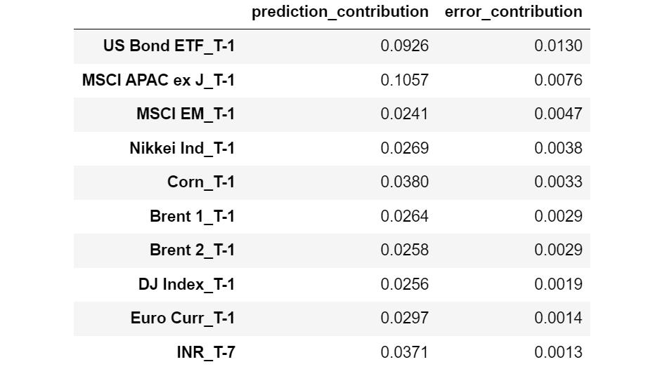
And now the features with the lowest Error Contribution:
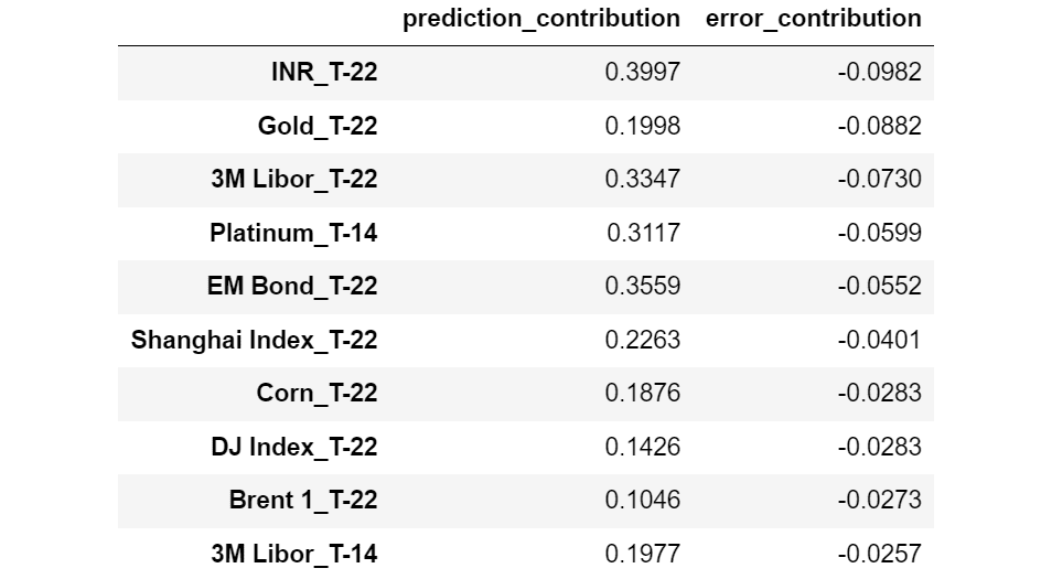
Features sorted by increasing Error Contribution. [Image by Author]
Interestingly, we may observe that all the features with higher Error Contribution are relative to T-1 (1 day before the observation moment), whereas almost all the features with smaller Error Contribution are relative to T-22 (22 days before the observation moment).
This seems to indicate that the most recent features are prone to overfitting, whereas the features more distant in time tend to generalize better.
Note that, without Error Contribution, we would never have known this insight.
Traditional Recursive Feature Elimination (RFE) methods are based on the removal of unimportant features. This is equivalent to removing the features with a small Prediction Contribution first.
However, based on what we said in the previous paragraph, it would make more sense to remove the features with the highest Error Contribution first.
To check whether our intuition is verified, let’s compare the two approaches:
- Traditional RFE: removing useless features first (lowest Prediction Contribution).
- Our RFE: removing harmful features first (highest Error Contribution).
Let’s see the results on the validation set:
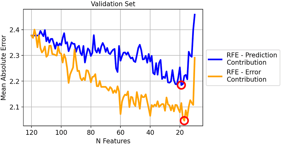
Mean Absolute Error of the two strategies on the validation set. [Image by Author]
The best iteration for each method has been circled: it’s the model with 19 features for the traditional RFE (blue line) and the model with 17 features for our RFE (orange line).
In general, it seems that our method works well: removing the feature with the highest Error Contribution leads to a consistently smaller MAE compared to removing the feature with the highest Prediction Contribution.
However, you may think that this works well just because we are overfitting the validation set. After all, we are interested in the result that we will obtain on the test set.
So let’s see the same comparison on the test set.
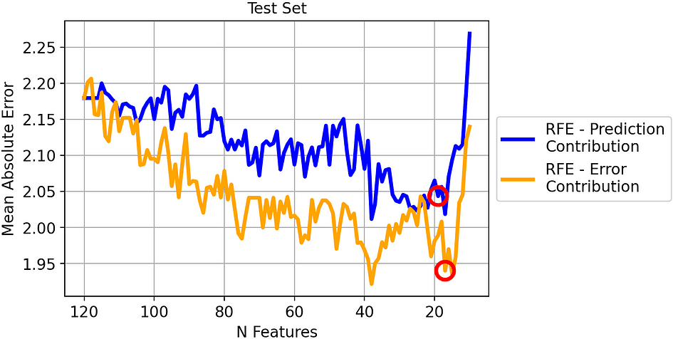
Mean Absolute Error of the two strategies on the test set. [Image by Author]
The result is similar to the previous one. Even if there is less distance between the two lines, the MAE obtained by removing the highest Error Contributor is clearly better than the MAE by obtained removing the lowest Prediction Contributor.
Since we selected the models leading to the smallest MAE on the validation set, let’s see their outcome on the test set:
- RFE-Prediction Contribution (19 features). MAE on test set: 2.04.
- RFE-Error Contribution (17 features). MAE on test set: 1.94.
So the best MAE using our method is 5% better compared to traditional RFE!
The concept of feature importance plays a fundamental role in machine learning. However, the notion of “importance” is often mistaken for “goodness”.
In order to distinguish between these two aspects we have introduced two concepts: Prediction Contribution and Error Contribution. Both concepts are based on the SHAP values of the validation dataset, and in the article we have seen the Python code to compute them.
We have also tried them on a real financial dataset (in which the task is predicting the price of Gold) and proved that Recursive Feature Elimination based on Error Contribution leads to a 5% better Mean Absolute Error compared to traditional RFE based on Prediction Contribution.
All the code used for this article can be found in this notebook.
Thank you for reading!
Samuele Mazzanti is Lead Data Scientist at Jakala and currently lives in Rome. He graduated in Statistics and his main research interests concern machine learning applications for the industry. He is also a freelance content creator.
Original. Reposted with permission.
- SEO Powered Content & PR Distribution. Get Amplified Today.
- PlatoData.Network Vertical Generative Ai. Empower Yourself. Access Here.
- PlatoAiStream. Web3 Intelligence. Knowledge Amplified. Access Here.
- PlatoESG. Carbon, CleanTech, Energy, Environment, Solar, Waste Management. Access Here.
- PlatoHealth. Biotech and Clinical Trials Intelligence. Access Here.
- Source: https://www.kdnuggets.com/your-features-are-important-it-doesnt-mean-they-are-good?utm_source=rss&utm_medium=rss&utm_campaign=your-features-are-important-it-doesnt-mean-they-are-good
- :has
- :is
- :not
- $UP
- 07
- 1
- 14
- 17
- 19
- 20k
- 22
- 7
- a
- About
- about IT
- above
- Absolute
- Accounts
- actually
- add
- additive
- After
- age
- ahead
- All
- allow
- almost
- also
- always
- am
- an
- and
- Another
- answer
- anything
- applications
- approaches
- ARE
- article
- AS
- aspect
- aspects
- asset
- Assets
- At
- author
- available
- average
- Bad
- based
- basic
- BE
- because
- been
- before
- beneficial
- BEST
- Better
- between
- Blue
- bond
- both
- bring
- Brings
- brought
- built
- but
- by
- calculate
- called
- CAN
- cannot
- carried
- case
- Changes
- check
- classification
- clearer
- clearly
- code
- compare
- compared
- comparison
- Compute
- concept
- concepts
- Concern
- Consider
- consistently
- contains
- content
- contrary
- contribution
- contributions
- contributor
- Correlation
- course
- creator
- Currently
- customer
- data
- data scientist
- datasets
- day
- Days
- difference
- different
- distance
- Distant
- distinction
- distinguish
- do
- Doesn’t
- done
- Dont
- down
- Drop
- due
- e
- each
- easily
- enough
- equal
- equally
- Equivalent
- error
- Errors
- Even
- exactly
- example
- Explainability
- explained
- expressed
- extract
- fact
- Feature
- Features
- final
- financial
- financial data
- First
- focused
- following
- For
- found
- freelance
- from
- full
- fundamental
- General
- generally
- get
- given
- goal
- Gold
- gold price
- good
- great
- Ground
- hand
- harm
- harmful
- Have
- he
- here
- High
- higher
- highest
- highly
- his
- How
- How To
- However
- HTTPS
- i
- ID
- idea
- identify
- if
- image
- importance
- important
- improve
- in
- In other
- Income
- Increase
- increasing
- indicate
- Indicator
- individual
- individuals
- industry
- Influential
- information
- insight
- insights
- instance
- instead
- interested
- interesting
- interests
- into
- introduced
- intuition
- IT
- iteration
- ITS
- Job
- just
- KDnuggets
- Know
- knowledge
- known
- largest
- lead
- leading
- Leads
- learning
- least
- less
- Library
- Line
- lines
- List
- Lives
- Look
- Lot
- lower
- lowest
- machine
- machine learning
- made
- Main
- make
- MAKES
- Making
- Matter
- Matters
- May..
- mean
- means
- method
- methods
- misconception
- model
- models
- moment
- more
- most
- much
- my
- Need
- negative
- never
- New
- note
- Notion
- now
- number
- observe
- observed
- obtain
- obtained
- of
- often
- on
- ONE
- or
- Orange
- order
- Other
- our
- out
- Outcome
- pandas
- part
- particularly
- People
- percentage
- performance
- period
- permission
- piece
- plato
- Plato Data Intelligence
- PlatoData
- plays
- positive
- possibly
- predict
- predicting
- prediction
- Predictions
- predictive
- presence
- previous
- price
- probably
- Problem
- procedure
- property
- proved
- proxy
- pushes
- Python
- question
- Read
- real
- really
- recent
- Recursive
- reduction
- regression
- relative
- relevant
- remaining
- removal
- remove
- Removed
- removing
- repeat
- research
- respective
- respectively
- result
- resulting
- Results
- return
- returns
- right
- Role
- rome
- ROW
- Said
- same
- say
- Scientist
- Second
- see
- seems
- seen
- selected
- sense
- Series
- set
- should
- sign
- similar
- Simple
- simply
- since
- single
- small
- smaller
- So
- some
- Someone
- specific
- statistics
- Step
- Steps
- stored
- strategies
- Take
- taken
- taking
- talking
- Target
- Task
- tell
- tends
- test
- than
- that
- The
- their
- Them
- then
- There.
- These
- they
- things
- think
- Third
- this
- those
- thousands
- three
- Through
- Thus
- time
- Time Series
- to
- Total
- traditional
- trained
- Training
- tried
- truth
- try
- trying
- two
- type
- us
- use
- used
- uses
- using
- validation
- Valuable
- value
- Values
- variable
- verified
- very
- vs
- want
- we
- WELL
- What
- when
- whereas
- whether
- which
- widely
- will
- with
- without
- words
- Work
- working
- works
- worse
- would
- you
- Your
- zephyrnet