This post is cowritten with Pramod Nayak, LakshmiKanth Mannem and Vivek Aggarwal from the Low Latency Group of LSEG.
Transaction cost analysis (TCA) is widely used by traders, portfolio managers, and brokers for pre-trade and post-trade analysis, and helps them measure and optimize transaction costs and the effectiveness of their trading strategies. In this post, we analyze options bid-ask spreads from the LSEG Tick History – PCAP dataset using Amazon Athena for Apache Spark. We show you how to access data, define custom functions to apply on data, query and filter the dataset, and visualize the results of the analysis, all without having to worry about setting up infrastructure or configuring Spark, even for large datasets.
Background
Options Price Reporting Authority (OPRA) serves as a crucial securities information processor, collecting, consolidating, and disseminating last sale reports, quotes, and pertinent information for US Options. With 18 active US Options exchanges and over 1.5 million eligible contracts, OPRA plays a pivotal role in providing comprehensive market data.
On February 5, 2024, the Securities Industry Automation Corporation (SIAC) is set to upgrade the OPRA feed from 48 to 96 multicast channels. This enhancement aims to optimize symbol distribution and line capacity utilization in response to escalating trading activity and volatility in the US options market. SIAC has recommended that firms prepare for peak data rates of up to 37.3 GBits per second.
Despite the upgrade not immediately altering the total volume of published data, it enables OPRA to disseminate data at a significantly faster rate. This transition is crucial for addressing the demands of the dynamic options market.
OPRA stands out as one the most voluminous feeds, with a peak of 150.4 billion messages in a single day in Q3 2023 and a capacity headroom requirement of 400 billion messages over a single day. Capturing every single message is critical for transaction cost analytics, market liquidity monitoring, trading strategy evaluation, and market research.
About the data
LSEG Tick History – PCAP is a cloud-based repository, exceeding 30 PB, housing ultra-high-quality global market data. This data is meticulously captured directly within the exchange data centers, employing redundant capture processes strategically positioned in major primary and backup exchange data centers worldwide. LSEG’s capture technology ensures lossless data capture and uses a GPS time-source for nanosecond timestamp precision. Additionally, sophisticated data arbitrage techniques are employed to seamlessly fill any data gaps. Subsequent to capture, the data undergoes meticulous processing and arbitration, and is then normalized into Parquet format using LSEG’s Real Time Ultra Direct (RTUD) feed handlers.
The normalization process, which is integral to preparing the data for analysis, generates up to 6 TB of compressed Parquet files per day. The massive volume of data is attributed to the encompassing nature of OPRA, spanning multiple exchanges, and featuring numerous options contracts characterized by diverse attributes. Increased market volatility and market making activity on the options exchanges further contribute to the volume of data published on OPRA.
The attributes of Tick History – PCAP enable firms to conduct various analyses, including the following:
- Pre-trade analysis – Evaluate potential trade impact and explore different execution strategies based on historical data
- Post-trade evaluation – Measure actual execution costs against benchmarks to assess the performance of execution strategies
- Optimized execution – Fine-tune execution strategies based on historical market patterns to minimize market impact and reduce overall trading costs
- Risk management – Identify slippage patterns, identify outliers, and proactively manage risks associated with trading activities
- Performance attribution – Separate the impact of trading decisions from investment decisions when analyzing portfolio performance
The LSEG Tick History – PCAP dataset is available in AWS Data Exchange and can be accessed on AWS Marketplace. With AWS Data Exchange for Amazon S3, you can access PCAP data directly from LSEG’s Amazon Simple Storage Service (Amazon S3) buckets, eliminating the need for firms to store their own copy of the data. This approach streamlines data management and storage, providing clients immediate access to high-quality PCAP or normalized data with ease of use, integration, and substantial data storage savings.
Athena for Apache Spark
For analytical endeavors, Athena for Apache Spark offers a simplified notebook experience accessible through the Athena console or Athena APIs, allowing you to build interactive Apache Spark applications. With an optimized Spark runtime, Athena helps the analysis of petabytes of data by dynamically scaling the number of Spark engines is less than a second. Moreover, common Python libraries such as pandas and NumPy are seamlessly integrated, allowing for the creation of intricate application logic. The flexibility extends to the importation of custom libraries for use in notebooks. Athena for Spark accommodates most open-data formats and is seamlessly integrated with the AWS Glue Data Catalog.
Dataset
For this analysis, we used the LSEG Tick History – PCAP OPRA dataset from May 17, 2023. This dataset comprises the following components:
- Best bid and offer (BBO) – Reports the highest bid and lowest ask for a security at a given exchange
- National best bid and offer (NBBO) – Reports the highest bid and lowest ask for a security across all exchanges
- Trades – Records completed trades across all exchanges
The dataset involves the following data volumes:
- Trades – 160 MB distributed across approximately 60 compressed Parquet files
- BBO – 2.4 TB distributed across approximately 300 compressed Parquet files
- NBBO – 2.8 TB distributed across approximately 200 compressed Parquet files
Analysis overview
Analyzing OPRA Tick History data for Transaction Cost Analysis (TCA) involves scrutinizing market quotes and trades around a specific trade event. We use the following metrics as part of this study:
- Quoted spread (QS) – Calculated as the difference between the BBO ask and the BBO bid
- Effective spread (ES) – Calculated as the difference between the trade price and the midpoint of the BBO (BBO bid + (BBO ask – BBO bid)/2)
- Effective/quoted spread (EQF) – Calculated as (ES / QS) * 100
We calculate these spreads before the trade and additionally at four intervals after the trade (just after, 1 second, 10 seconds, and 60 seconds after the trade).
Configure Athena for Apache Spark
To configure Athena for Apache Spark, complete the following steps:
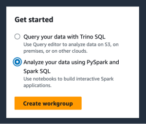
- On the Athena console, under Get started, select Analyze your data using PySpark and Spark SQL.
- If this is your first time using Athena Spark, choose Create workgroup.
- For Workgroup name¸ enter a name for the workgroup, such as
tca-analysis. - In the Analytics engine section, select Apache Spark.
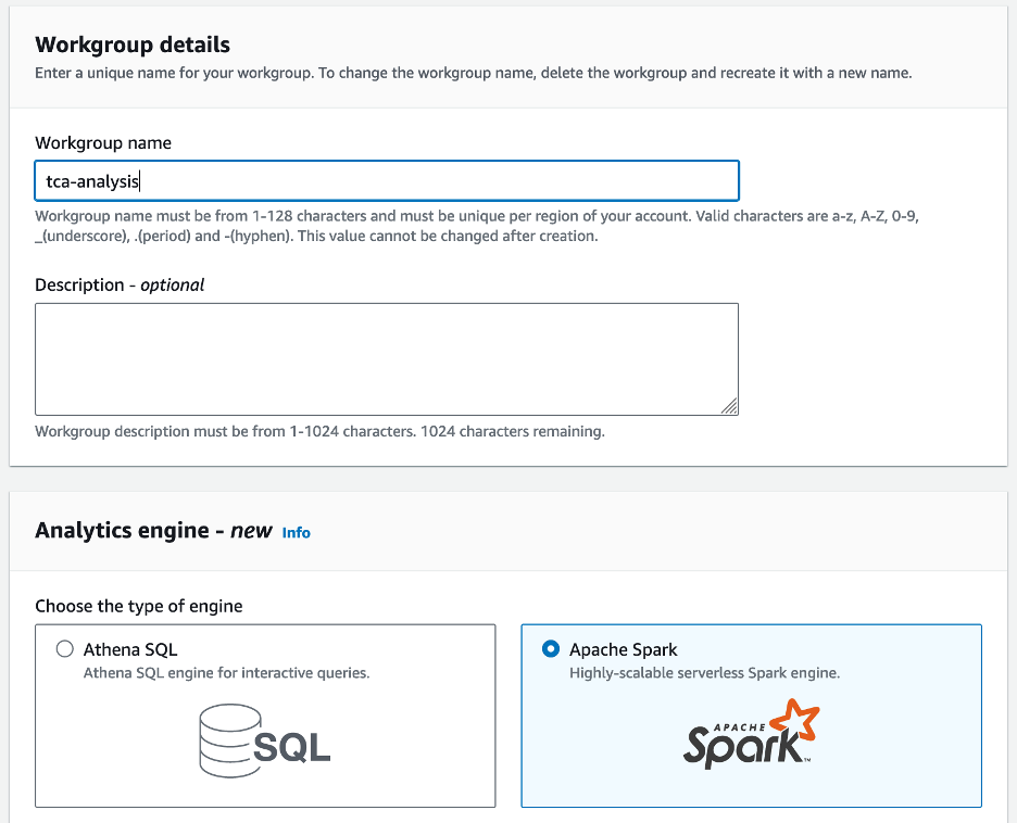
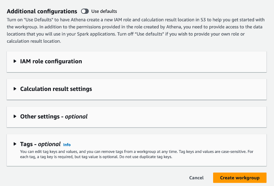
- In the Additional configurations section, you can choose Use defaults or provide a custom AWS Identity and Access Management (IAM) role and Amazon S3 location for calculation results.
- Choose Create workgroup.
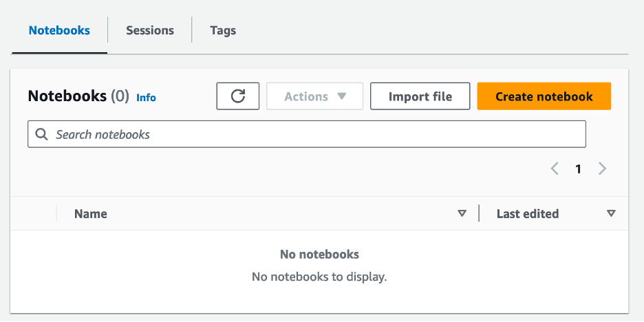
- After you create the workgroup, navigate to the Notebooks tab and choose Create notebook.
- Enter a name for your notebook, such as
tca-analysis-with-tick-history. - Choose Create to create your notebook.
Launch your notebook
If you have already created a Spark workgroup, select Launch notebook editor under Get started.
![]()
After your notebook is created, you will be redirected to the interactive notebook editor.
![]()
Now we can add and run the following code to our notebook.
Create an analysis
Complete the following steps to create an analysis:
- Import common libraries:
- Create our data frames for BBO, NBBO, and trades:
- Now we can identify a trade to use for transaction cost analysis:
We get the following output:
We use the highlighted trade information going forward for the trade product (tp), trade price (tpr), and trade time (tt).
- Here we create a number of helper functions for our analysis
- In the following function, we create the dataset that contains all the quotes before and after the trade. Athena Spark automatically determines how many DPUs to launch for processing our dataset.
- Now let’s call the TCA analysis function with the information from our selected trade:
Visualize the analysis results
Now let’s create the data frames we use for our visualization. Each data frame contains quotes for one of the five time intervals for each data feed (BBO, NBBO):
In the following sections, we provide example code to create different visualizations.
Plot QS and NBBO before the trade
Use the following code to plot the quoted spread and NBBO before the trade:
![]()
Plot QS for each market and NBBO after the trade
Use the following code to plot the quoted spread for each market and NBBO immediately after the trade:
![]()
Plot QS for each time interval and each market for BBO
Use the following code to plot the quoted spread for each time interval and each market for BBO:
![]()
Plot ES for each time interval and market for BBO
Use the following code to plot the effective spread for each time interval and market for BBO:
Plot EQF for each time interval and market for BBO
Use the following code to plot the effective/quoted spread for each time interval and market for BBO:
Athena Spark calculation performance
When you run a code block, Athena Spark automatically determines how many DPUs it requires to complete the calculation. In the last code block, where we call the tca_analysis function, we are actually instructing Spark to process the data, and we then convert the resulting Spark dataframes into Pandas dataframes. This constitutes the most intensive processing part of the analysis, and when Athena Spark runs this block, it shows the progress bar, elapsed time, and how many DPUs are processing data currently. For example, in the following calculation, Athena Spark is utilizing 18 DPUs.
![]()
When you configure your Athena Spark notebook, you have the option of setting the maximum number of DPUs that it can use. The default is 20 DPUs, but we tested this calculation with 10, 20, and 40 DPUs to demonstrate how Athena Spark automatically scales to run our analysis. We observed that Athena Spark scales linearly, taking 15 minutes and 21 seconds when the notebook was configured with a maximum of 10 DPUs, 8 minutes and 23 seconds when the notebook was configured with 20 DPUs, and 4 minutes and 44 seconds when the notebook was configured with 40 DPUs. Because Athena Spark charges based on DPU usage, at a per-second granularity, the cost of these calculations is similar, but if you set a higher maximum DPU value, Athena Spark can return the result of the analysis much faster. For more details on Athena Spark pricing please click here.
Conclusion
In this post, we demonstrated how you can use high-fidelity OPRA data from LSEG’s Tick History-PCAP to perform transaction cost analytics using Athena Spark. The availability of OPRA data in a timely manner, complemented with accessibility innovations of AWS Data Exchange for Amazon S3, strategically reduces the time to analytics for firms looking to create actionable insights for critical trading decisions. OPRA generates about 7 TB of normalized Parquet data each day, and managing the infrastructure to provide analytics based on OPRA data is challenging.
Athena’s scalability in handling large-scale data processing for Tick History – PCAP for OPRA data makes it a compelling choice for organizations seeking swift and scalable analytics solutions in AWS. This post shows the seamless interaction between the AWS ecosystem and Tick History-PCAP data and how financial institutions can take advantage of this synergy to drive data-driven decision-making for critical trading and investment strategies.
About the Authors
![]() Pramod Nayak is the Director of Product Management of the Low Latency Group at LSEG. Pramod has over 10 years of experience in the financial technology industry, focusing on software development, analytics, and data management. Pramod is a former software engineer and passionate about market data and quantitative trading.
Pramod Nayak is the Director of Product Management of the Low Latency Group at LSEG. Pramod has over 10 years of experience in the financial technology industry, focusing on software development, analytics, and data management. Pramod is a former software engineer and passionate about market data and quantitative trading.
![]() LakshmiKanth Mannem is a Product Manager in the Low Latency Group of LSEG. He focuses on data and platform products for the low-latency market data industry. LakshmiKanth helps customers build the most optimal solutions for their market data needs.
LakshmiKanth Mannem is a Product Manager in the Low Latency Group of LSEG. He focuses on data and platform products for the low-latency market data industry. LakshmiKanth helps customers build the most optimal solutions for their market data needs.
![]() Vivek Aggarwal is a Senior Data Engineer in the Low Latency Group of LSEG. Vivek works on developing and maintaining data pipelines for processing and delivery of captured market data feeds and reference data feeds.
Vivek Aggarwal is a Senior Data Engineer in the Low Latency Group of LSEG. Vivek works on developing and maintaining data pipelines for processing and delivery of captured market data feeds and reference data feeds.
![]() Alket Memushaj is a Principal Architect in the Financial Services Market Development team at AWS. Alket is responsible for technical strategy, working with partners and customers to deploy even the most demanding capital markets workloads to the AWS Cloud.
Alket Memushaj is a Principal Architect in the Financial Services Market Development team at AWS. Alket is responsible for technical strategy, working with partners and customers to deploy even the most demanding capital markets workloads to the AWS Cloud.
- SEO Powered Content & PR Distribution. Get Amplified Today.
- PlatoData.Network Vertical Generative Ai. Empower Yourself. Access Here.
- PlatoAiStream. Web3 Intelligence. Knowledge Amplified. Access Here.
- PlatoESG. Carbon, CleanTech, Energy, Environment, Solar, Waste Management. Access Here.
- PlatoHealth. Biotech and Clinical Trials Intelligence. Access Here.
- Source: https://aws.amazon.com/blogs/big-data/mastering-market-dynamics-transforming-transaction-cost-analytics-with-ultra-precise-tick-history-pcap-and-amazon-athena-for-apache-spark/
- :has
- :is
- :not
- :where
- $UP
- 1
- 10
- 100
- 12
- 15%
- 150
- 16
- 160
- 17
- 19
- 20
- 200
- 2023
- 2024
- 23
- 27
- 30
- 300
- 40
- 400
- 60
- 7
- 750
- 8
- 90
- a
- About
- access
- accessed
- accessibility
- accessible
- across
- active
- activity
- actual
- actually
- add
- Additionally
- addressing
- ADvantage
- After
- against
- Aggarwal
- aims
- All
- Allowing
- already
- Amazon
- Amazon Athena
- Amazon Web Services
- an
- analyses
- analysis
- Analytical
- analytics
- analyze
- analyzing
- and
- any
- Apache
- Apache Spark
- APIs
- Application
- applications
- Apply
- approach
- approximately
- arbitrage
- arbitration
- ARE
- around
- AS
- ask
- assess
- associated
- At
- attributes
- authority
- automatically
- Automation
- availability
- available
- AWS
- Backup
- bar
- based
- BE
- because
- before
- benchmarks
- BEST
- between
- bid
- Billion
- Block
- brokers
- build
- but
- by
- calculate
- calculated
- calculation
- call
- CAN
- Capacity
- capital
- Capital Markets
- capture
- captured
- Capturing
- catalog
- Centers
- challenging
- channels
- characterized
- charges
- choice
- Choose
- clients
- Cloud
- code
- Collecting
- Common
- compelling
- complete
- Completed
- components
- comprehensive
- comprises
- Conduct
- configured
- configuring
- Console
- consolidating
- contains
- contracts
- contribute
- convert
- CORPORATION
- Cost
- Costs
- cowritten
- create
- created
- creation
- critical
- crucial
- Currently
- custom
- Customers
- Dash
- data
- data centers
- data engineer
- Data Exchange
- data management
- data processing
- data storage
- data-driven
- datasets
- day
- Decision Making
- decisions
- Default
- define
- delivery
- demanding
- demands
- demonstrate
- demonstrated
- deploy
- details
- determines
- developing
- Development
- development team
- difference
- different
- directly
- Director
- distributed
- distribution
- diverse
- double
- drive
- dynamic
- dynamically
- dynamics
- each
- ease
- ease of use
- ecosystem
- editor
- Effective
- effectiveness
- eligible
- eliminating
- employed
- employing
- enable
- enables
- encompassing
- endeavors
- Engine
- engineer
- Engines
- enhancement
- ensures
- Enter
- escalating
- Ether (ETH)
- evaluate
- evaluation
- Even
- Event
- Every
- example
- exchange
- Exchanges
- execution
- experience
- explore
- express
- extends
- faster
- Featuring
- February
- Fig
- Files
- fill
- filter
- financial
- Financial institutions
- financial services
- financial technology
- firms
- First
- first time
- five
- Flexibility
- focuses
- focusing
- following
- For
- format
- Former
- Forward
- four
- FRAME
- from
- function
- functions
- further
- gaps
- generates
- get
- given
- Global
- global market
- Go
- going
- gps
- Group
- Handling
- Have
- having
- he
- headroom
- helps
- high-quality
- higher
- highest
- Highlighted
- historical
- history
- housing
- How
- How To
- http
- HTTPS
- IAM
- identify
- Identity
- if
- immediate
- immediately
- Impact
- import
- in
- Including
- increased
- industry
- information
- Infrastructure
- innovations
- insights
- institutions
- integral
- integrated
- integration
- interaction
- interactive
- into
- intricate
- investment
- involves
- IT
- jpg
- just
- large
- large-scale
- Last
- Latency
- launch
- less
- libraries
- Line
- Liquidity
- location
- logic
- looking
- Low
- lowest
- maintaining
- major
- MAKES
- Making
- manage
- management
- manager
- Managers
- managing
- manner
- many
- Market
- Market Data
- market impact
- market research
- market volatility
- market-making
- Markets
- massive
- Mastering
- maximum
- May..
- measure
- message
- messages
- meticulous
- meticulously
- Metrics
- million
- minimize
- minutes
- monitoring
- more
- Moreover
- most
- much
- multiple
- name
- Nature
- Navigate
- Need
- needs
- None
- notebook
- notebooks
- number
- numerous
- numpy
- observed
- of
- offer
- Offers
- on
- ONE
- optimal
- Optimize
- optimized
- Option
- Options
- or
- organizations
- our
- out
- output
- over
- overall
- own
- pandas
- part
- partners
- passionate
- patterns
- Peak
- per
- perform
- performance
- pivotal
- platform
- plato
- Plato Data Intelligence
- PlatoData
- plays
- please
- plot
- portfolio
- portfolio managers
- positioned
- Post
- post-trade
- potential
- Precision
- Prepare
- preparing
- price
- pricing
- primary
- Principal
- process
- processes
- processing
- Processor
- Product
- product management
- product manager
- Products
- Progress
- provide
- providing
- published
- Python
- Q3
- quantitative
- quantity
- query
- quotes
- Rate
- Rates
- Read
- real
- real-time
- recommended
- records
- Red
- reduce
- reduces
- reference
- refinitiv
- Reporting
- Reports
- repository
- requirement
- requires
- research
- response
- responsible
- result
- resulting
- Results
- return
- risks
- Role
- Run
- runs
- sale
- Scalability
- scalable
- scales
- scaling
- seamless
- seamlessly
- Second
- seconds
- Section
- sections
- Securities
- security
- seeking
- select
- selected
- senior
- separate
- serves
- Services
- set
- setting
- show
- Shows
- significantly
- similar
- Simple
- simplified
- single
- slippage
- Software
- software development
- Software Engineer
- Solutions
- sophisticated
- spanning
- Spark
- specific
- spread
- Spreads
- stands
- Steps
- storage
- store
- Strategically
- strategies
- Strategy
- streamlines
- Study
- subsequent
- such
- SWIFT
- symbol
- synergy
- Take
- taking
- team
- Technical
- techniques
- Technology
- tested
- than
- that
- The
- the information
- their
- Them
- then
- These
- this
- Through
- tick
- time
- timely
- timestamp
- Title
- to
- Total
- tp
- TPR
- trade
- Traders
- trades
- Trading
- Trading Strategies
- trading strategy
- transaction
- transaction costs
- transforming
- transition
- Ultra
- under
- undergoes
- upgrade
- us
- Usage
- use
- used
- uses
- using
- Utilizing
- value
- various
- visualization
- visualize
- Volatility
- volume
- volumes
- was
- we
- web
- web services
- when
- which
- widely
- will
- with
- within
- without
- Workgroup
- working
- works
- worldwide
- worry
- X
- years
- you
- Your
- zephyrnet