مصنف کی طرف سے تصویر
If you’re familiar with the unsupervised learning paradigm, you’d have come across dimensionality reduction and the algorithms used for dimensionality reduction such as the پرنسپل اجزاء کا تجزیہ (PCA). Datasets for machine learning typically contain a large number of features, but such high-dimensional feature spaces are not always helpful.
In general, all the features are نوٹ equally important and there are certain features that account for a large percentage of variance in the dataset. Dimensionality reduction algorithms aim to reduce the dimension of the feature space to a fraction of the original number of dimensions. In doing so, the features with high variance are still retained—but are in the transformed feature space. And principal component analysis (PCA) is one of the most popular dimensionality reduction algorithms.
In this tutorial, we’ll learn how principal component analysis (PCA) works and how to implement it using the scikit-learn library.
Before we go ahead and implement principal component analysis (PCA) in scikit-learn, it’s helpful to understand how PCA works.
As mentioned, principal component analysis is a dimensionality reduction algorithm. Meaning it reduces the dimensionality of the feature space. But how does it achieve this reduction?
The motivation behind the algorithm is that there are certain features that capture a large percentage of variance in the original dataset. So it’s important to find the directions of maximum variance in the dataset. These directions are called اہم اجزاء. And PCA is essentially a projection of the dataset onto the principal components.
So how do we find the principal components?
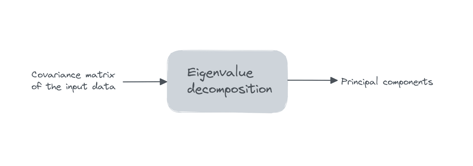
Suppose the data matrix X is of dimensions num_observations x num_features, we perform eigenvalue decomposition پر ہم آہنگی میٹرکس ایکس کا
If the features are all zero mean, then the covariance matrix is given by X.T X. Here, X.T is the transpose of the matrix X. If the features are not all zero mean initially, we can subtract the mean of column i from each entry in that column and compute the covariance matrix. It’s simple to see that the covariance matrix is a square matrix of order نمبر_خصوصیات.
مصنف کی طرف سے تصویر
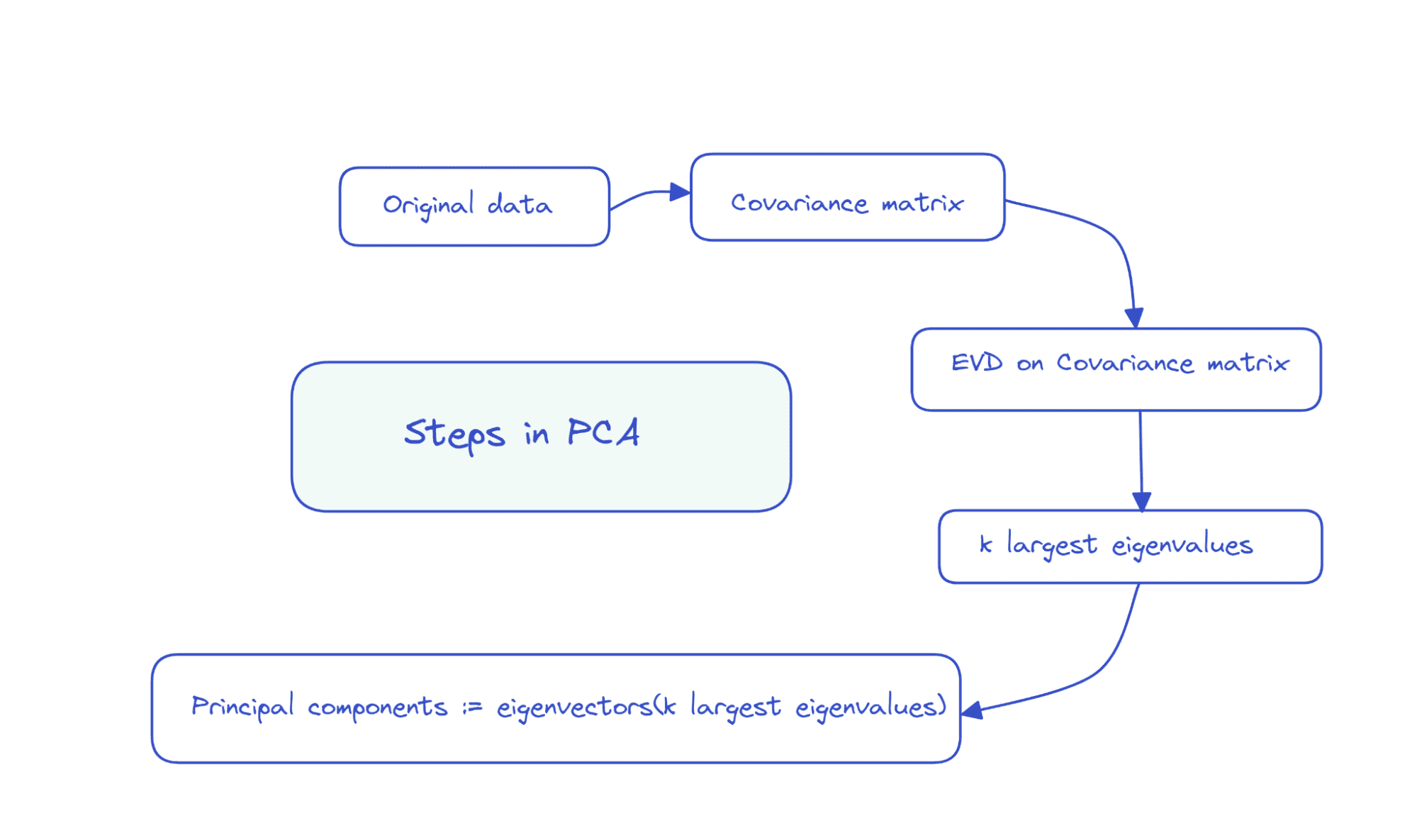
The first k principal components are the eigenvectors کے مطابق k largest eigenvalues.
So the steps in PCA can be summarized as follows:
مصنف کی طرف سے تصویر
Because the covariance matrix is a symmetric and positive semi-definite, the eigendecomposition takes the following form:
X.T X = D Λ D.T
Where, D is the matrix of eigenvectors and Λ is a diagonal matrix of eigenvalues.
Another matrix factorization technique that can be used to compute principal components is singular value decomposition or SVD.
Singular value decomposition (SVD) is defined for all matrices. Given a matrix X, SVD of X gives: X = U Σ V.T. Here, U, Σ, and V are the matrices of left singular vectors, singular values, and right singular vectors, respectively. V.T. is the transpose of V.
So the SVD of the covariance matrix of X is given by:

Comparing the equivalence of the two matrix decompositions:

We have the following:

There are computationally efficient algorithms for calculating the SVD of a matrix. The scikit-learn implementation of PCA also uses SVD under the hood to compute the principal components.
Now that we’ve learned the basics of principal component analysis, let’s proceed with the scikit-learn implementation of the same.
مرحلہ 1 - ڈیٹاسیٹ لوڈ کریں۔
To understand how to implement principal component analysis, let’s use a simple dataset. In this tutorial, we’ll use the wine dataset available as part of scikit-learn’s ڈیٹاسیٹس ماڈیول.
Let’s start by loading and preprocessing the dataset:
from sklearn import datasets
wine_data = datasets.load_wine(as_frame=True)
df = wine_data.data
It has 13 features and 178 records in all.
print(df.shape)
Output >> (178, 13)
print(df.info())
Output >>

RangeIndex: 178 entries, 0 to 177
Data columns (total 13 columns): # Column Non-Null Count Dtype --- ------ -------------- ----- 0 alcohol 178 non-null float64 1 malic_acid 178 non-null float64 2 ash 178 non-null float64 3 alcalinity_of_ash 178 non-null float64 4 magnesium 178 non-null float64 5 total_phenols 178 non-null float64 6 flavanoids 178 non-null float64 7 nonflavanoid_phenols 178 non-null float64 8 proanthocyanins 178 non-null float64 9 color_intensity 178 non-null float64 10 hue 178 non-null float64 11 od280/od315_of_diluted_wines 178 non-null float64 12 proline 178 non-null float64
dtypes: float64(13)
memory usage: 18.2 KB
None
Step 2 – Preprocess the Dataset
As a next step, let’s preprocess the dataset. The features are all on different scales. To bring them all to a common scale, we’ll use the StandardScaler that transforms the features to have zero mean and unit variance:
from sklearn.preprocessing import StandardScaler
std_scaler = StandardScaler()
scaled_df = std_scaler.fit_transform(df)
Step 3 – Perform PCA on the Preprocessed Dataset
To find the principal components, we can use the PCA class from scikit-learn’s سڑن ماڈیول.
Let’s instantiate a PCA object by passing in the number of principal components n_components to the constructor.
The number of principal components is the number of dimensions that you’d like to reduce the feature space to. Here, we set the number of components to 3.
from sklearn.decomposition import PCA
pca = PCA(n_components=3)
pca.fit_transform(scaled_df)
Instead of calling the fit_transform() method, you can also call fit() اس کے بعد transform() طریقہ.
Notice how the steps in principal component analysis such as computing the covariance matrix, performing eigendecomposition or singular value decomposition on the covariance matrix to get the principal components have all been abstracted away when we use scikit-learn’s implementation of PCA.
Step 4 – Examining Some Useful Attributes of the PCA Object
The PCA instance pca that we created has several useful attributes that help us understand what is going on under the hood.
وصف components_ stores the directions of maximum variance (the principal components).
print(pca.components_)
Output >>
[[ 0.1443294 -0.24518758 -0.00205106 -0.23932041 0.14199204 0.39466085 0.4229343 -0.2985331 0.31342949 -0.0886167 0.29671456 0.37616741 0.28675223] [-0.48365155 -0.22493093 -0.31606881 0.0105905 -0.299634 -0.06503951 0.00335981 -0.02877949 -0.03930172 -0.52999567 0.27923515 0.16449619 -0.36490283] [-0.20738262 0.08901289 0.6262239 0.61208035 0.13075693 0.14617896 0.1506819 0.17036816 0.14945431 -0.13730621 0.08522192 0.16600459 -0.12674592]]
We mentioned that the principal components are directions of maximum variance in the dataset. But how do we measure how much of the total variance is captured in the number of principal components we just chose?
۔ explained_variance_ratio_ attribute captures the ratio of the total variance each principal component captures. Sowe can sum up the ratios to get the total variance in the chosen number of components.
print(sum(pca.explained_variance_ratio_))
Output >> 0.6652996889318527
Here, we see that three principal components capture over 66.5% of total variance in the dataset.
Step 5 – Analyzing the Change in Explained Variance Ratio
We can try running principal component analysis by varying the number of components n_components.
import numpy as np
nums = np.arange(14)
var_ratio = []
for num in nums: pca = PCA(n_components=num) pca.fit(scaled_df) var_ratio.append(np.sum(pca.explained_variance_ratio_))
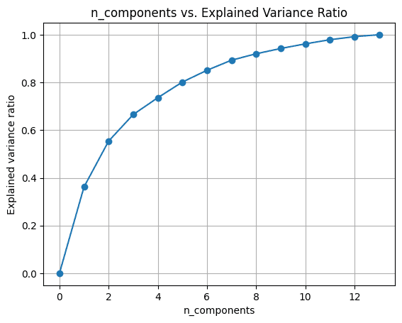
To visualize the explained_variance_ratio_ for the number of components, let’s plot the two quantities as shown:
import matplotlib.pyplot as plt plt.figure(figsize=(4,2),dpi=150)
plt.grid()
plt.plot(nums,var_ratio,marker='o')
plt.xlabel('n_components')
plt.ylabel('Explained variance ratio')
plt.title('n_components vs. Explained Variance Ratio')
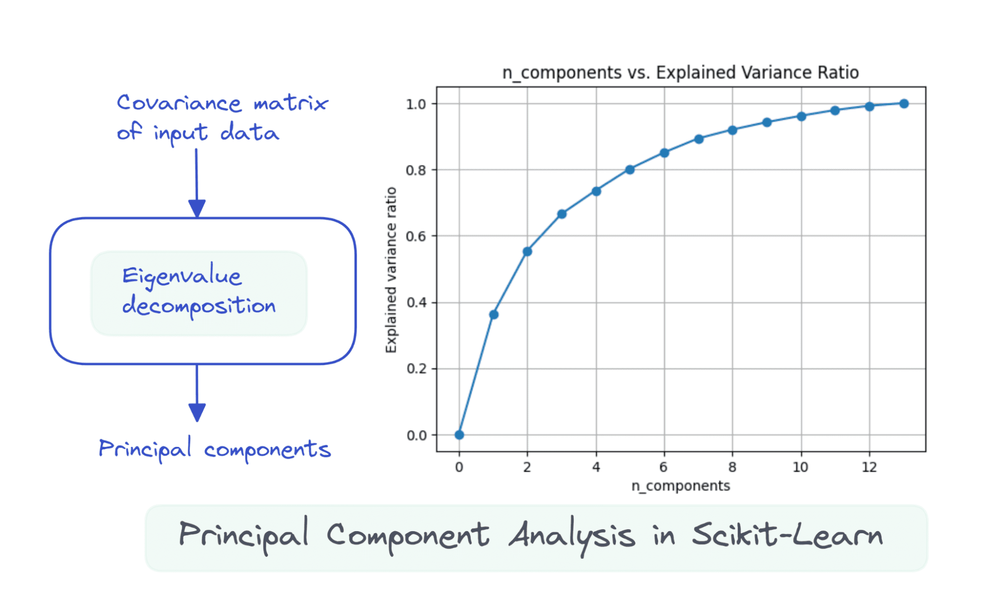
When we use all the 13 components, the explained_variance_ratio_ is 1.0 indicating that we’ve captured 100% of the variance in the dataset.
In this example, we see that with 6 principal components, we’ll be able to capture more than 80% of variance in the input dataset.
I hope you’ve learned how to perform principal component analysis using built-in functionality in the scikit-learn library. Next, you can try to implement PCA on a dataset of your choice. If you’re looking for good datasets to work with, check out this list of websites to find datasets for your data science projects.
ہے [1] Computational Linear Algebra, fast.ai
بالا پریا سی ہندوستان سے ایک ڈویلپر اور تکنیکی مصنف ہے۔ وہ ریاضی، پروگرامنگ، ڈیٹا سائنس، اور مواد کی تخلیق کے چوراہے پر کام کرنا پسند کرتی ہے۔ اس کی دلچسپی اور مہارت کے شعبوں میں DevOps، ڈیٹا سائنس، اور قدرتی زبان کی پروسیسنگ شامل ہیں۔ وہ پڑھنے، لکھنے، کوڈنگ اور کافی سے لطف اندوز ہوتی ہے! فی الحال، وہ سیکھنے اور اپنے علم کو ڈویلپر کمیونٹی کے ساتھ بانٹنے کے لیے ٹیوٹوریلز، کیسے گائیڈز، رائے کے ٹکڑوں اور مزید بہت کچھ لکھ کر کام کر رہی ہے۔
- SEO سے چلنے والا مواد اور PR کی تقسیم۔ آج ہی بڑھا دیں۔
- پلیٹوآئ اسٹریم۔ ویب 3 ڈیٹا انٹیلی جنس۔ علم میں اضافہ۔ یہاں تک رسائی حاصل کریں۔
- ایڈریین ایشلے کے ساتھ مستقبل کا نقشہ بنانا۔ یہاں تک رسائی حاصل کریں۔
- PREIPO® کے ساتھ PRE-IPO کمپنیوں میں حصص خریدیں اور بیچیں۔ یہاں تک رسائی حاصل کریں۔
- ماخذ: https://www.kdnuggets.com/2023/05/principal-component-analysis-pca-scikitlearn.html?utm_source=rss&utm_medium=rss&utm_campaign=principal-component-analysis-pca-with-scikit-learn
- : ہے
- : ہے
- : نہیں
- $UP
- 1
- 10
- 11
- 12
- 13
- 14
- 66
- 7
- 8
- 9
- a
- قابلیت
- اکاؤنٹ
- حاصل
- کے پار
- آگے
- مقصد
- شراب
- یلگورتم
- یلگوردمز
- تمام
- بھی
- ہمیشہ
- تجزیہ
- تجزیہ
- اور
- کیا
- علاقوں
- AS
- At
- اوصاف
- تصنیف
- دستیاب
- دور
- مبادیات
- BE
- رہا
- پیچھے
- لانے
- تعمیر میں
- لیکن
- by
- حساب
- فون
- کہا جاتا ہے
- بلا
- کر سکتے ہیں
- قبضہ
- قبضہ
- کچھ
- تبدیل
- چیک کریں
- انتخاب
- کا انتخاب کیا
- منتخب کیا
- طبقے
- کوڈنگ
- کالم
- کالم
- کس طرح
- کامن
- کمیونٹی
- جزو
- اجزاء
- کمپیوٹنگ
- کمپیوٹنگ
- مواد
- مواد کی تخلیق
- اسی کے مطابق
- بنائی
- مخلوق
- اس وقت
- اعداد و شمار
- ڈیٹا سائنس
- ڈیٹاسیٹس
- کی وضاحت
- ڈیولپر
- DevOps
- مختلف
- طول و عرض
- طول و عرض
- ہدایات
- do
- کرتا
- کر
- ہر ایک
- ہنر
- اندراج
- یکساں طور پر
- بنیادی طور پر
- جانچ کر رہا ہے
- مثال کے طور پر
- مہارت
- وضاحت کی
- واقف
- فاسٹ
- نمایاں کریں
- خصوصیات
- مل
- پہلا
- پیچھے پیچھے
- کے بعد
- مندرجہ ذیل ہے
- کے لئے
- فارم
- کسر
- سے
- فعالیت
- جنرل
- حاصل
- دی
- فراہم کرتا ہے
- Go
- جا
- اچھا
- ہدایات
- ہے
- مدد
- مدد گار
- اس کی
- یہاں
- ہائی
- ہڈ
- امید ہے کہ
- کس طرح
- کیسے
- HTML
- HTTPS
- i
- if
- پر عملدرآمد
- نفاذ
- درآمد
- اہم
- in
- شامل
- بھارت
- اشارہ کرتے ہیں
- ابتدائی طور پر
- ان پٹ
- مثال کے طور پر
- دلچسپی
- چوراہا
- IT
- صرف
- KDnuggets
- علم
- زبان
- بڑے
- سب سے بڑا
- جانیں
- سیکھا ہے
- سیکھنے
- چھوڑ دیا
- لائبریری
- کی طرح
- لنکڈ
- لسٹ
- ll
- لوڈ
- لوڈ کر رہا ہے
- تلاش
- مشین
- مشین لرننگ
- ریاضی
- matplotlib
- میٹرکس
- زیادہ سے زیادہ
- مطلب
- مطلب
- پیمائش
- یاد داشت
- ذکر کیا
- طریقہ
- ماڈیول
- زیادہ
- سب سے زیادہ
- سب سے زیادہ مقبول
- پریرتا
- بہت
- قدرتی
- قدرتی زبان
- قدرتی زبان عملیات
- اگلے
- تعداد
- عجیب
- اعتراض
- of
- on
- ایک
- رائے
- or
- حکم
- اصل
- باہر
- پیداوار
- پر
- پیرا میٹر
- حصہ
- پاسنگ
- فیصد
- انجام دینے کے
- کارکردگی کا مظاہرہ
- ٹکڑے ٹکڑے
- پلاٹا
- افلاطون ڈیٹا انٹیلی جنس
- پلیٹو ڈیٹا
- مقبول
- مثبت
- پرنسپل
- پروسیسنگ
- پروگرامنگ
- پروجیکشن
- تناسب
- پڑھنا
- ریکارڈ
- کو کم
- کم
- کمی
- بالترتیب
- ٹھیک ہے
- چل رہا ہے
- s
- اسی
- پیمانے
- ترازو
- سائنس
- سائنٹ سیکھنا
- دیکھنا
- مقرر
- کئی
- شکل
- اشتراک
- وہ
- دکھایا گیا
- سادہ
- واحد
- So
- کچھ
- خلا
- خالی جگہیں
- چوک میں
- شروع کریں
- مرحلہ
- مراحل
- ابھی تک
- پردہ
- اس طرح
- لیتا ہے
- ٹیکنیکل
- سے
- کہ
- ۔
- مبادیات
- ان
- تو
- وہاں.
- یہ
- اس
- تین
- کرنے کے لئے
- کل
- تبدیل
- کوشش
- سبق
- سبق
- دو
- عام طور پر
- کے تحت
- سمجھ
- یونٹ
- غیر زیر نگرانی تعلیم
- us
- استعمال
- استعمال کی شرائط
- استعمال کیا جاتا ہے
- کا استعمال کرتے ہوئے
- قیمت
- اقدار
- vs
- we
- کیا
- کیا ہے
- جب
- وکیپیڈیا
- شراب
- ساتھ
- کام
- کام کر
- کام کرتا ہے
- مصنف
- تحریری طور پر
- X
- آپ
- اور
- زیفیرنیٹ
- صفر